How Row Goal shapes your SQL Server query strategy by hunting for pierogis

The Wroclaw Connection

SQLDay 2026 took place this week, from May 11th to 13th, in Wroclaw. Among the featured speakers was Erik Darling, who delivered both a main session and a full-day workshop dedicated to SQL Server performance. During his presentations, he emphasized a concept that is not always widely understood, known as the Row Goal.

The purpose of this article is to recap Erik’s key observations and to introduce this topic, which can serve as a powerful lever for query optimization.

A quick culinary detour and why pierogis matter

In order to understand the explanations below, one key concept must be understood: the Pierogi.

“Pierogi are filled dumplings made from unleavened dough, popular in Polish cuisine and enjoyed worldwide, with various savory and sweet fillings” [1], [2].

To be honest, this has nothing to do with our technical topic, but this dish discovered during this trip is so good that I simply had to include it in this blog.

Filling the aisles and designing our database

In this article, we will use a custom-made database simulating a Polish supermarket selling pierogis. Unfortunately, there aren’t many left, and the product distribution is not uniform. In fact, pierogis account for much less than 1% of the supermarket’s total stock.
Here is the script to create the DB, along with its article reference table and inventory:

USE master;
GO

IF EXISTS (SELECT * FROM sys.databases WHERE name = 'PierogiMart')
    DROP DATABASE PierogiMart;
GO

CREATE DATABASE PierogiMart;
GO

USE PierogiMart;
GO

CREATE TABLE Articles (
    ArticleID INT IDENTITY(1,1) PRIMARY KEY,
    ArticleName VARCHAR(50) NOT NULL,
    Price DECIMAL(10, 2) NOT NULL
);

CREATE TABLE Inventory (
    ReferenceID INT IDENTITY(1,1) PRIMARY KEY,
    ArticleID INT NOT NULL,
    ValidityDate DATETIME NOT NULL,
    Quantity INT NOT NULL,
    CONSTRAINT FK_Article FOREIGN KEY (ArticleID) REFERENCES Articles(ArticleID)
);
GO

INSERT INTO Articles (ArticleName, Price)
VALUES 
('Pierogi', 12.50),
('Pasta', 8.00),
('Sandwich', 6.50),
('Quiche', 9.00);
GO

INSERT INTO Inventory (ArticleID, ValidityDate, Quantity)
SELECT TOP 100000 
    2, 
    DATEADD(DAY, ABS(CHECKSUM(NEWID())) % 365, '2025-01-01'), 
    ABS(CHECKSUM(NEWID())) % 100
FROM sys.all_columns a CROSS JOIN sys.all_columns b;

INSERT INTO Inventory (ArticleID, ValidityDate, Quantity)
SELECT TOP 10000 
    3, 
    DATEADD(DAY, ABS(CHECKSUM(NEWID())) % 365, '2025-01-01'), 
    ABS(CHECKSUM(NEWID())) % 100
FROM sys.all_columns a CROSS JOIN sys.all_columns b;

INSERT INTO Inventory (ArticleID, ValidityDate, Quantity)
SELECT TOP 50000 
    4, 
    DATEADD(DAY, ABS(CHECKSUM(NEWID())) % 365, '2025-01-01'), 
    ABS(CHECKSUM(NEWID())) % 100
FROM sys.all_columns a CROSS JOIN sys.all_columns b;

INSERT INTO Inventory (ArticleID, ValidityDate, Quantity)
SELECT TOP 10 
    1, 
    '2026-12-31', 
    5
FROM sys.all_columns;
GO

We are also including a few indexes to simulate a real-world use case and to support our queries, ensuring we get realistic execution plans:

CREATE NONCLUSTERED INDEX IDX_INV_QUANT ON [dbo].[Inventory] ([Quantity]) include (ArticleID)

CREATE NONCLUSTERED INDEX IDX_INV_VALIDITY on [dbo].[Inventory] ([ValidityDate]) include (ArticleID)

CREATE NONCLUSTERED INDEX IDX_INV_ART on [dbo].[Inventory] (ArticleID)

What exactly is a Row Goal?

Normally, the SQL Server optimizer seeks to minimize the total cost of processing all data for a query. However, if it knows that you only need a specific number of rows (for example, via a TOP, FAST(N), or EXISTS clause), it changes its strategy.

The Row Goal is this specific row target that pushes the optimizer to favor a plan capable of delivering the first few rows as quickly as possible, even if that same plan would be catastrophic for processing the entire table.

TOP(N): Hunting for the best Pierogi

To illustrate the definition above, let’s search for the pierogis with the furthest expiration dates.
Note that the IDX_INV_VALIDITY index supports this query:

SELECT 
    A.ArticleName, 
    A.Price, 
    I.ValidityDate
FROM Articles A
INNER JOIN Inventory I ON A.ArticleID = I.ArticleID
WHERE A.ArticleName = 'Pierogi'
order by I.ValidityDate desc;

SELECT top 10
    A.ArticleName, 
    A.Price, 
    I.ValidityDate
FROM Articles A
INNER JOIN Inventory I ON A.ArticleID = I.ArticleID
WHERE A.ArticleName = 'Pierogi'
order by I.ValidityDate desc

The difference between these two queries is that one requests only the first 10 rows, while the other requests all matching rows. However, this simple distinction is not merely applied when displaying the results; this condition is pushed deeper into the execution plan to influence the choice of operators (Nested Loop, Hash Join, Merge Join) further down the tree.

For the first query, here is the resulting plan:

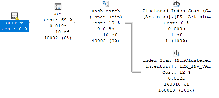
As we can see, the optimizer chose a Hash Join given the volume of data to be joined. A Hash Match implies that all the data must be read in order to produce the desired result.

For the second query, here is the execution plan:

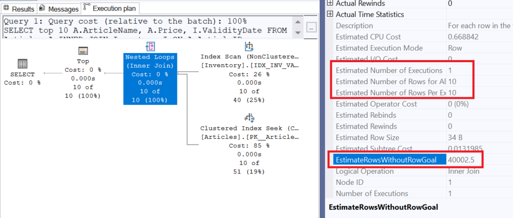
We can see that this time, the optimizer chose a Nested Loop, which takes each row from the reference table (Inventory) and joins them with the Articles table. This operation can be very time-consuming if a large number of rows must be processed. However, this is where EstimateRowsWithoutRowGoal comes into play. The value of this property is 40’002.5; this means that in a case where a subset of rows was not specifically required, the optimizer would have estimated the number of rows returned by this operator at that value. We can see, however, that the estimation actually used is 10 rows for one execution, a value clearly derived from the TOP(10).

In summary, adding the TOP(10) allowed the optimizer to use a less expensive join for a small amount of data, even though the TOP operator is located at the very end of the execution plan (since a plan is read from right to left).

EXISTS: The search for the first match

As explained previously, the EXISTS clause has a cardinality of 1 because the very first row meeting the internal condition is enough to validate the case. This triggers a Row Goal, as the optimizer must estimate how many rows it will need to read to satisfy (or not) this condition.

Note: In cases where the condition is never met, the optimizer’s plan can become highly inefficient; for full details, see Erik Darling’s blog [here].

We will now observe this behavior with the following query, varying the internal condition of the EXISTS clause by testing one highly selective (discriminant) case and another much less so.

SELECT 
    A.ArticleName, 
    A.Price
FROM Articles A
WHERE not EXISTS (
    SELECT 1/0
    FROM Inventory I 
    WHERE I.ArticleID = A.ArticleID 
    AND I.Quantity > 10 -- vs 98
);

As you may have noticed, I am looking here for products that maintain a certain quantity for every possible consumption date. My goal, of course, is to avoid depleting the stocks of these excellent Polish pierogis so that everyone can enjoy them!

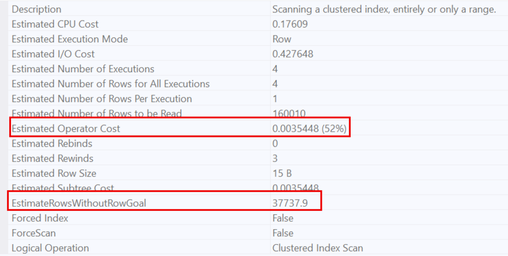
The case where we want to ensure that all existing quantities for an item are greater than 10 is very difficult to satisfy; based on the statistics available to the optimizer, all items have 10 or more units in stock, except for the pierogis!
Since this condition is so widespread, the optimizer knows it will have to scan a large number of rows to find a single case where the condition is not met. This is why it opts for a Scan. This behavior is evidenced by the estimated number of rows to be read (160’010, which represents the entire table).

On the other hand, for a very restrictive condition (quantity > 98), the optimizer recognizes that this condition is highly selective. This is why it favors a Nested Loop, estimating that only 1’608 rows will be necessary to prove the non-existence of the condition.

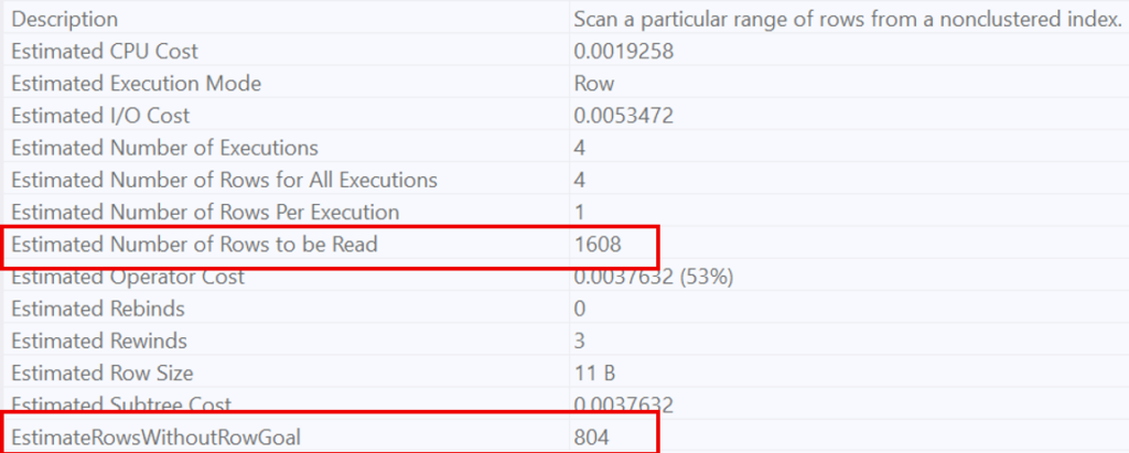
In summary, EXISTS forces the optimizer to estimate the number of rows required to find a single occurrence that proves whether a condition is met or not, thereby triggering a local optimization of the execution plan.

OPTION(FAST N): Manually steering the engine

The OPTION(FAST N) hint allows you to manually introduce the Row Goal concept into a query. This hint does not limit the total number of results returned; instead, it optimizes the execution plan to retrieve the first N rows as quickly as possible (potentially at the expense of performance for the remaining rows).

In our example below, we have two identical queries retrieving items with a quantity greater than 10. However, the second one uses an execution plan optimized to return the first row as fast as possible (just to make sure no one steals the last available pierogi from the top of the pile!).

select * from Inventory i
where i.Quantity > 10 
order by i.ArticleID

select * from Inventory i
where i.Quantity > 10 
order by i.ArticleID option(fast 1)

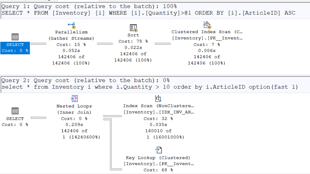
Once again, the plans diverge. To retrieve a single row, the IDX_INV_ART index (which already contains sorted ArticleIDs) is used. It performs a Seek on the smallest ArticleID to check if it satisfies the condition of having a quantity greater than 10.

However, by enabling SET STATISTICS TIME ON, we can see that the second execution plan is slower than the first when returning all requested rows (250ms vs. 204ms). While the gap is not massive due to the small table size, the difference is nonetheless observable.

Wrapping up and how to survive the Row Goal gamble

To conclude, the Row Goal is a double-edged sword; brilliant when you only need a quick glimpse of your data, but it can become a real performance trap if the optimizer’s “bet” fails.

Fortunately, if you find that SQL Server is making bad decisions by being too optimistic, you can take back control. By using the hint OPTION (USE HINT ('DISABLE_OPTIMIZER_ROWGOAL')), you force the optimizer to stop daydreaming and focus on the actual cost of the query. It’s the ultimate tool to ensure your execution plan doesn’t end up as messy as a dropped plate of pierogis!