
For my first blog post at dbi services, I think it could be a good opportunity to begin by discussing around SQL Server 2014, Hekaton memory optimized tables, and hash indexes. When you create a memory optimized table you have to consider the number of buckets that you have to reserve for its associated hash index. It’s an important aspect of configuration because after creating your table, you cannot change the number of buckets without recreating it.
For the SQL Server database administrators world, it is not usual because with other ordinary indexes (clustered, nonclustered indexes) or other special indexes (xml or spatial indexes) this parameter does not exist. Furthermore, Microsoft recommends to reserve a number of buckets equal at least two times the number of distinct values in the table! The first time I read the documentation I asked myself a few questions:
- Why reserve a fixed number of buckets?
- Why round the number of buckets to the power of 2?
In order to find the answers, I first had to understand how a hash index works.
Let’s start from a basic definition of a hash table: it is a data structure used to implement an unsorted associative data array that can map a key to a value. To compute this key a hash function is used. The hash result is then stored into an array of buckets as shown to figure 1 (simplified schema).
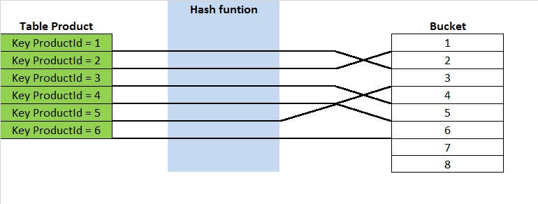
Notice that the hashing keys are not sorted. For lookup operations it does not matter, but for range value scans the hash index does not perform well. In the hash table world, the ideal situation is one key for one unique bucket to allow constant time for lookups, but in reality it is not the case because of hash collisions (two distinct pieces of data can have the same hash value). However, the hash function should be efficient enough to spread keys into buckets uniformly to avoid this phenomenon as much as possible.
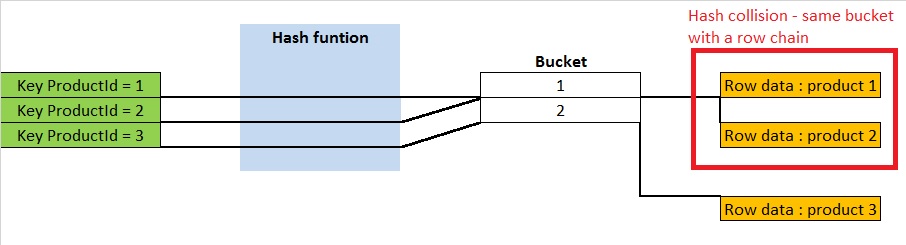
There are several strategies to resolve hash collisions and the lack of buckets. SQL Server uses a method that consists of a separated chaining. When a hash collision occurs or when the number of buckets is not sufficient, the row data is added to the row chain for the selecting bucket. In consequence, the cost of the table operation is that of scanning the number of entries in the row chain of the selecting bucket for the concerned index key. If the distribution is sufficiently uniform, the average cost of a lookup depends only on the average number of keys per bucket also called the load factor. The load factor is the number of total entries divided by the number of buckets. The larger the load factor, the more the hash table will be slow. It means for a fixed number of buckets the time for lookups will grow with the number of entries.
Now let’s start with a practical example of a memory-optimized table :
We create a simple memory optimized table with two columns and 1000 buckets to store the hash index entries. After creating this table, we can see the number of buckets allocated and we notice the final number is not the same, but rounded to the nearest power of two.
![]()
This fact is very interesting because using a power of two to determine the position of the bucket pointer in the array is very efficient. Generally, with hash tables the hash function process is done in two steps to determine the index in the buckets array:
- hash value = hash function (key)
- position in the array = hash value % array size
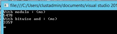
The modulo operator in the case could be very expensive and can fortunately be replaced by a bitwise AND operator (because the array size is a power of two) which reduces the operation to masking and improves speed. To verify, we can do a simple test with a console application in C#:
By executing this console application on my dev environment (Intel Core i7-3610QM 2.30 GHz), we can notice that the bitwise and function performs faster than the modulo function for an iteration of 1 billion:
Then we can play with different combination of data rows and hash index buckets to understand why the number of bucket is very important.
Test 1: Filling up the table with 500 distinct rows and 1024 buckets
By using the DMV sys.dm_db_xtp_hash_index_stats we can see useful information about buckets usage.
![]()
We retrieve the total number of buckets allocated for the index hash equal to 1024. Furthermore, we notice that we have 545 empty buckets and in consequence 1024 – 545 = 479 buckets in use. Normally, with a perfect distribution of key values in the bucket array, we should have 500 buckets in use, but we notice that we certainly already have some hash collisions. We can verify this in the value of the column max_chain_length which tells us there is at least one bucket with a row chain length of 2. In other words, we have at least one bucket that contains two rows with the same index hash. Notice that the load factor is equal to 500 / 1024 = 0.49
Test 2: Filling up the memory-optimized table with a load factor of 3. We will insert 3072 rows for a total of bucket count equal to 1024
![]()
As expected, all buckets are used (empty_bucket_count = 0). We have an average row chain length of 3 (avg_chain_length = 3) in the bucket array equal to the load factor. Some of the rows chain lengths are equal to five, certainly due to a hash collision (max_chain_length = 5).
Test 3: Filling up the memory-optimized table with duplicate rows
Before filling up the table, some changes in the schema are required. Let’s create a second non-unique hash index (ix_OrderDate):
Then we can fill up the table with 500 rows that contain some duplicate rows:
Here is an overview of the number of duplicates rows in the table:
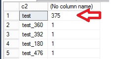
We can now check how the buckets are used for the two hash indexes:
We retrieve the same number of used buckets for the primary hash index key (545) as first tests. This is because the hash function used by SQL Server is deterministic. The same index key is always mapped to the same bucket in the array. The index key is relatively well distributed. However, we can see a different result for the second hash index. We only have 119 buckets in use to store 500 rows. Furthermore, we notice that the maximum row chain length is very high and corresponds in fact to the number of duplicates values we inserted (375).
Test 4: Filling up the table with an insufficient number of buckets to uniformly store the hash indexes
For this last test, we will use 10 buckets to store 8192 distinct rows (a load factor = 819).
![]()
In this case, only one bucket is used (no empty buckets) and the value of the avg_chain_length and the max_chain_length column are pretty close. This is an indication of a lack of buckets with a big row chain.
In this post, we have seen the basic concepts of the hash table, the importance of a correct configuration of the buckets and how to use the dynamic management view sys.dm_db_xtp_index_hash_stats to get useful statistics for hash indexes.
By David Barbarin
![Thumbnail [60x60]](https://www.dbi-services.com/blog/wp-content/uploads/2022/12/microsoft-square.png)
![Thumbnail [90x90]](https://www.dbi-services.com/blog/wp-content/uploads/2022/09/DDI_web-min-scaled.jpg)