Introduction
In the last blog post we did setup a LAB with a DVDRental database mixed with Netflix data on top which we created some embeddings hosted on the same tables thanks to pgvector. In this second part, we will start to look at improving query execution time with some indexes before extending on the rest of the AI workflow.
But first let’s talk about why developing those skills is so important.
Rollback 40 years ago. Back then we had applications storing data on ISAM databases. Basically flat files. Then we created this thing called SQL and the RDBMS with ACID properties to make it run. This moved the logic from the application only to have a bit in both sides. If you are a DBA with “some experience” you might remember the days when producing stored procedures, triggers with complex logic was complementary to the application code that DEVs couldn’t or wouldn’t change… the issue being that the code on the database side was harder to maintain.
Then 15-20 years ago we started to use ORMs everywhere and moved the logic from the RDBMS side to the ORM or app. This enabled to partially decouple the app from its backend database server and allow for having more sources (NOSQL DBMS) but also migrate easier from one system to another. This is why the lasts years we have a lot of migrations towards other RDBMS, it is today more easy than ever, “you just” have to add a new connector without changing the app. As DBA we went from tuning a lot of SQL code to almost fraction of it because the ORMs became better and better.
Where do I go with all of that ?
Well, with AI, the logic is going to leave the ORMs and app part and only be in the AI model tuned for your business. What does that mean ? It means that you will have an easier access to all of your data. You won’t have to wait for a team of developer to develop the panel of dashboards and reports you want in the app, you just going to ask the AI the data in the way you want it and it will just know of to connect to your database and build the query.
My point : consequence of that is that the databases are going to be hammered more than ever and most of the limitations that your going to have is the design choice of your database backend and your AI workflow. Not the app anymore. Learning how to optimize AI workflow and data retrieval will be key for the future.
So after this intro, let’s dive into those new PostgreSQL vector indexes a bit…
As a reminder here is the Git repo with the instructions and all the links for the other parts of this series.
Part 1 : pgvector, a guide for DBA – Part1 LAB DEMO
Part 3 : pgvector, a guide for DBA – Part3 AI Agent and workflows
Part 4 : pgvector, a guide for DBA – Part 4 AI Workflows Best practices ( not released yet )
Index types in pgvector
pgvector supports natively two types of indexes that are approximate nearest neighbor (ANN) indexes. Unlike other indexes in PostgreSQL like B-tree or GiST, the ANN indexes trade some recall accuracy for query speed. What does it mean? It means that index searches with ANN won’t necessarily return the same return as a sequential scan.
HNSW Index
The Hierarchical Navigable Small World (HNSW) index builds a multi‐layer graph where each node (a vector) is connected to a fixed number of neighbors. During a search, the algorithm starts at the top (sparse) layer and “zooms in” through lower layers to quickly converge on the nearest neighbors.
- Key parameters:
- m: Maximum number of links per node (default is 16).
- ef_construction: Candidate list size during index build (default is 64).
- ef_search: Size of the dynamic candidate list during query (default is 40; can be tuned per query).
- Characteristics & Use Cases:
- Excellent query speed and high recall.
- Suitable for workloads where fast similarity search is critical—even if build time and memory consumption are higher.
Here is an example of a query and some index to support it.
CREATE INDEX film_embedding_idx
ON public.film USING hnsw (embedding vector_l2_ops)

CREATE INDEX netflix_shows_embedding_idx
ON public.netflix_shows USING hnsw (embedding vector_l2_ops)
Here is the execution plan of this query :
-- (Using existing HNSW index on film.embedding)
EXPLAIN ANALYZE
SELECT film_id, title
FROM film
ORDER BY embedding <-> '[-0.0060701305,-0.008093507...]' --choose any embedding from the table
LIMIT 5;

Limit  (cost=133.11..133.12 rows=5 width=27) (actual time=7.498..7.500 rows=5 loops=1)
   ->  Sort  (cost=133.11..135.61 rows=1000 width=27) (actual time=7.497..7.497 rows=5 loops=1)
         Sort Key: ((embedding <-> '[-0.0060701305,-0.008093507,-0.0019467601,0.015574081,0.012467623,0.032596912,-0.0284>
         Sort Method: top-N heapsort  Memory: 25kB
         ->  Seq Scan on film  (cost=0.00..116.50 rows=1000 width=27) (actual time=0.034..7.243 rows=1000 loops=1)
 Planning Time: 0.115 ms
 Execution Time: 7.521 ms
(7 rows)
IVFFlat Index
IVFFlat (Inverted File with Flat compression) first partitions the vector space into clusters (lists) by running a clustering algorithm (typically k-means). Each vector is assigned to the nearest cluster (centroid). At query time, only a subset (controlled by the number of probes) of the closest clusters are scanned rather than the entire dataset
- Key parameters:
- lists: Number of clusters created at index build time (a good starting point is rows/1000 for up to 1M rows or sqrt(rows) for larger datasets).
- probes: Number of clusters to search during a query (default is 1; higher values improve recall at the cost of speed).
- Characteristics & Use Cases:
- Faster index build and smaller index size compared to HNSW.
- May yield slightly lower recall or slower query performance if too few probes are used.
- Best used when the dataset is relatively static (since the clusters are built only once).
CREATE INDEX film_embedding_ivfflat_idx
ON film USING ivfflat (embedding vector_l2_ops) WITH (lists = 100);
With the same query as before we have now this execution plan :
 Limit  (cost=27.60..43.40 rows=5 width=27) (actual time=0.288..0.335 rows=5 loops=1)
   ->  Index Scan using film_embedding_ivfflat_idx on film  (cost=27.60..3188.50 rows=1000 width=27) (actual time=0.286..>
         Order By: (embedding <-> '[-0.0060701305,-0.008093507,-0.0019467601,0.015574081,0.012467623,0.032596912,-0.02841>
 Planning Time: 0.565 ms
 Execution Time: 0.375 ms
(5 rows)- Example Query:
After setting the number of probes, you can run:
SET ivfflat.probes = 5;

    -- New execution plan
    Limit  (cost=133.11..133.12 rows=5 width=27) (actual time=7.270..7.272 rows=5 loops=1)
   ->  Sort  (cost=133.11..135.61 rows=1000 width=27) (actual time=7.268..7.269 rows=5 loops=1)
         Sort Key: ((embedding <-> '[-0.0060701305,-0.008093507,-0.0019467601,0.015574081,0.012467623,0.032596912,-0.0284>
         Sort Method: top-N heapsort  Memory: 25kB
         ->  Seq Scan on film  (cost=0.00..116.50 rows=1000 width=27) (actual time=0.054..6.984 rows=1000 loops=1)
 Planning Time: 0.140 ms
 Execution Time: 7.293 ms
(7 rows)
By changing the number of probes :
SET ivfflat.probes = 10;

   -- New execution plan
    Limit  (cost=104.75..120.17 rows=5 width=27) (actual time=0.459..0.499 rows=5 loops=1)
   ->  Index Scan using film_embedding_ivfflat_idx on film  (cost=104.75..3188.50 rows=1000 width=27) (actual time=0.458.>
         Order By: (embedding <-> '[-0.0060701305,-0.008093507,-0.0019467601,0.015574081,0.012467623,0.032596912,-0.02841>
 Planning Time: 0.153 ms
 Execution Time: 0.524 ms
(5 rows)
Understanding Lists and Probes in IVFFlat Indexes
When you create an IVFFlat index, you specify a parameter called lists. This parameter determines how many clusters (or “lists”) the index will divide your entire dataset into. Essentially, during index build time, the algorithm runs a clustering process (commonly using k-means) on your vectors and assigns each vector to the nearest cluster centroid.
For example, if you set lists = 100 during index creation, the entire dataset is divided into 100 clusters. Then at query time, setting probes = 1 means only the single cluster whose centroid is closest to the query vector is examined. Increasing probes (say, to 10) instructs PostgreSQL to examine 10 clusters—improving recall by reducing the chance of missing the true nearest neighbors at the cost of extra computation. Lists define the overall structure of the index, while probes control the breadth of search within that structure at runtime. They are related but serve different purposes: one is fixed at build time, and the other is adjustable at query time.
A higher number of lists means that each cluster is smaller. This can lead to faster candidate comparisons because fewer vectors lie in any one cluster, but if you over-partition the data, you might risk missing close vectors that fall on the boundary between clusters.
The probes parameter is a query-time setting that tells the index how many of these pre-computed clusters to search when processing a query.
Tuning Index Parameters
- HNSW:
- Query time: Adjust
hnsw.ef_searchto trade-off between speed and recall. Higher values improve recall (more candidate vectors examined) but slow down queries. - Build time: Increasing
moref_constructioncan improve the quality (recall) of the index, but also increase build time and memory consumption.
- Query time: Adjust
- IVFFlat:
- Lists: Choosing the right number of clusters is essential. Use rules like rows/1000 for smaller datasets or sqrt(rows) for larger ones.
- Probes: Increase the number of probes (using
SET ivfflat.probes = value;) if recall is too low. This will widen the search among clusters at the cost of increased query time.
And then comes DiskANN Indexes
DiskANN was originally a research project from Microsoft Research and is open-sourced on GitHub. It uses a graph (like HNSW) but optimized for disk access patterns (paging neighbors in and out). Based on Microsoft research the team from Timescale produced pgvectorscale which is an open-source PostgreSQL extension that builds on top of the pgvector extension to provide DiskANN-based indexing for high-performance vector similarity search.
It introduces a new StreamingDiskANN index inspired by Microsoft’s DiskANN algorithm, along with Statistical Binary Quantization (SBQ) for compressing vector data.
What is the big deal with DiskANN and StreamingDiskANN ? Well, the main idea behind it is to avoid having all the information in memory (like with HNSW and IVFFlat) and store the bulk of the index on disk and only load small, relevant parts into memory when needed. This eliminates the memory bottleneck with massive datasets and provide a sub-linear scaling with RAM usage. DiskANN can handle billion‐scale datasets without demanding terabytes of memory.
These innovations significantly improve query speed and storage efficiency for embedding (vector) data in Postgres. In practice, PostgreSQL with pgvector + pgvectorscale has been shown to achieve dramatically lower query latencies and higher throughput compared to specialized vector databases!
How to install pgvectorscale ?
Building from Source: pgvectorscale is written in Rust (using the PGRX framework) and can be compiled and installed into an existing PostgreSQL instance (GitHub – timescale/pgvectorscale: A complement to pgvector for high performance, cost efficient vector search on large workloads.) (GitHub – timescale/pgvectorscale: A complement to pgvector for high performance, cost efficient vector search on large workloads.).
For my setup, I adapted the installation procedure provided to be able to install the pgvectorscale extension on my custom setup :
curl --proto '=https' --tlsv1.2 -sSf https://sh.rustup.rs | sh

cargo install --force --locked cargo-pgrx --version 0.12.5

cargo pgrx init --pg17 /u01/app/postgres/product/17/db_2/bin/pg_config

cd /tmp
git clone --branch 0.6.0  https://github.com/timescale/pgvectorscale
cd pgvectorscale/pgvectorscale
cargo pgrx install --release
CREATE EXTENSION IF NOT EXISTS vectorscale CASCADE;CREATE INDEX netflix_embedding_idx
ON netflix_shows
USING diskann (embedding vector_l2_ops);
I am planning to perform a full benchmark comparison with different solutions and with a AI/LLM as client in order to measure the real impact on performance. In the meantime, you might wanna check the Timescale benchmark on the matter compared to Pinecone: Pgvector vs. Pinecone: Vector Database Comparison | Timescale
To make a quick summary of the characteristics of each index types :
| Index Type | Build Speed | Query Speed | Memory Usage | Maintenance | Selectivity/Accuracy |
|---|---|---|---|---|---|
| DiskANN (pgvectorscale) | Fast | Fastest | Low (uses disk) | Updatable (no rebuild) | High (approximate, tuned) |
| HNSW (pgvector) | Fast | Fast | High (in-memory) | Updatable (no rebuild) | High (approximate) |
| IVFFlat (pgvector) | Fastest | Slowest | Low/Moderate | Rebuild required after bulk change | Moderat-high (tuning dependant) |
| B-TREE | Very fast | Small | low | none | Exact |
Operators, Selectivity & Hybrid Search Optimizations
If you are familiar with RDBMS query tuning optimizations, you might already understand the importance of the selectivity of your data.

In the RDBMS world, if we index the color of the tree, “yellow” is selective, “green” is not. It is not the index that matters it’s the selectivity of the data you’re looking for to the optimizer’s eyes (yes an optimizer has eyes, and he sees everything!).
When performing and hybrid SQL/similarity search we will typically try to filter a subset of rows on top of which we will execute a similarity vector search. I kind of didn’t talk about that but it is one of the most important parts of having vectors in a database! You can look for similarities! What does it mean ?!
It allows you to run an approximate search against a table. That’s it. When you are looking for something that kind of reassembles what input you provide… In the first part of this blog series, I briefly explain the fact that embeddings encapsulate meanings into numbers in the form of a vector. The closer two vectors in that context, the more they are the same. In my example, we use text embedding to look for similarities but you have models that work with videos, sound, or images as well.
For example, Deezer is using “FLOW” which is looking for your music taste of the playlist you saved and is proposing similar songs in addition to the ones you already like. In addition, it can compare your taste profile with your mood (inputs or events of you skipping songs fast).
Contrary to the classic indexes in PostgreSQL, vector indexes are by definition non-deterministic.
They use approximations to narrow down the search space. In the index search process, the Recall measures the fraction of the data that is returned to be true. Higher recall means better precision at the cost of speed and index size. Running the same vector multiple times might slightly return different rankings or even different subset of the nearest neighbors. This means that DBAs have to play with some index parameters like ef_search, ef_construction, m ( for HNSW ) or lists and probes ( for IVFFlat).
Playing with those parameters will help find the balance between speed and recall.
One advice would be to start with the default and combine with deterministic filters before touching any parameters. In most cases having 99% or 98% of recall is really fine. But like in the deterministic world, understanding your data is key.
Here in my LAB example, I use the description field in both netflix_shows and film tables. Although the methodology I am using is good enough I would say, the results generated might be completely off because the film table of the dvdrental database are not real movies and their description are not reliable which is not the case for the netflix_shows table. So when I am looking at the user average embedding on their top movies rented… I am going to compare things that might not be comparable, which will provide an output that is probably not meaningful.
Quick reminder, when looking for similarities you can use two operators in your SQL query : <-> (Euclidean): is Sensitive to magnitude differences. <=> (Cosine): Focuses on the angle of vectors, often yielding more semantically relevant results for text embeddings.
Which one should you use and when ?
Well, initially embedding are created by embedding models, they define the usage of the magnitude in the vector or not. If your model is not using the magnitude parameter to encompass additional characteristics, then only the angle > Cosine operator makes sense. The Euclidean operator would work but is suboptimal since you try to compute something that isn’t there. You should rely on the embedding model documentation to make your choice or just test if the results you are having differ in meaning.
In my example, I use text-embedding-ada-002 model, where the direction (angle) is the primary carrier of semantic meaning.
Note that those operators are used to define your indexes ! Like for JSONB queries in PostgreSQL, not using the proper operator can make the optimizer not choose the index and use a sequential scan instead.
One other important aspect a DBA has to take into consideration is that the PostgreSQL optimizer is still being used and has still the same behaviour which is one of the strength of using pgvector. You already know the beast !
For example depending on the query and the data set size, the optimizer would find more cost-effective to run a sequential scan than using an index, my sample dvdrental data set is not really taking advantage of the indexes benefits in most cases. The tables have only 1000 and 8000 rows.
Let’s look at some interesting cases. This first query is not using an index. Here we are looking for the top 5 Netflix shows whose vector embeddings are most similar to a customer profile embedding which is calculated be the average of film embeddings the customer 524 has rented.
postgres=# \c dvdrental
You are now connected to database "dvdrental" as user "postgres".
dvdrental=# WITH customer_profile AS (
  SELECT AVG(f.embedding) AS profile_embedding
  FROM rental r
  JOIN inventory i ON r.inventory_id = i.inventory_id
  JOIN film f ON i.film_id = f.film_id
  WHERE r.customer_id = 524
)
SELECT n.title,
       n.description,
       n.embedding <-> cp.profile_embedding AS distance
FROM netflix_shows n, customer_profile cp
WHERE n.embedding IS NOT NULL
ORDER BY n.embedding <=> cp.profile_embedding
LIMIT 5;
            title             |                                                                     description                                                                      |      distance
------------------------------+------------------------------------------------------------------------------------------------------------------------------------------------------+---------------------
 Alarmoty in the Land of Fire | While vacationing at a resort, an ornery and outspoken man is held captive by a criminal organization.                                               |  0.4504742864770678
 Baaghi                       | A martial artist faces his biggest test when he has to travel to Bangkok to rescue the woman he loves from the clutches of his romantic rival.       |  0.4517695114131648
 Into the Badlands            | Dreaming of escaping to a distant city, a ferocious warrior and a mysterious boy tangle with territorial warlords and their highly trained killers.  | 0.45256925901147355
 Antidote                     | A tough-as-nails treasure hunter protects a humanitarian doctor as she tries to cure a supernatural disease caused by a mysterious witch.            |  0.4526900472984078
 Duplicate                    | Hilarious mix-ups and deadly encounters ensue when a convict seeks to escape authorities by assuming the identity of his doppelgänger, a perky chef. | 0.45530040371443564
(5 rows)

dvdrental=# explain analyze WITH customer_profile AS (
  SELECT AVG(f.embedding) AS profile_embedding
  FROM rental r
  JOIN inventory i ON r.inventory_id = i.inventory_id
  JOIN film f ON i.film_id = f.film_id
  WHERE r.customer_id = 524
)
SELECT n.title,
       n.description,
       n.embedding <=> cp.profile_embedding AS distance
FROM netflix_shows n, customer_profile cp
WHERE n.embedding IS NOT NULL
ORDER BY n.embedding <=> cp.profile_embedding
LIMIT 5;
                                                                    QUERY PLAN
--------------------------------------------------------------------------------------------------------------------------------------------------
 Limit  (cost=1457.26..1457.27 rows=5 width=173) (actual time=40.076..40.081 rows=5 loops=1)
   ->  Sort  (cost=1457.26..1479.27 rows=8807 width=173) (actual time=40.075..40.079 rows=5 loops=1)
         Sort Key: ((n.embedding <-> (avg(f.embedding))))
         Sort Method: top-N heapsort  Memory: 27kB
         ->  Nested Loop  (cost=471.81..1310.97 rows=8807 width=173) (actual time=1.822..38.620 rows=8807 loops=1)
               ->  Aggregate  (cost=471.81..471.82 rows=1 width=32) (actual time=1.808..1.812 rows=1 loops=1)
                     ->  Nested Loop  (cost=351.14..471.74 rows=25 width=18) (actual time=0.938..1.479 rows=19 loops=1)
                           ->  Hash Join  (cost=350.86..462.01 rows=25 width=2) (actual time=0.927..1.431 rows=19 loops=1)
                                 Hash Cond: (i.inventory_id = r.inventory_id)
                                 ->  Seq Scan on inventory i  (cost=0.00..70.81 rows=4581 width=6) (actual time=0.006..0.262 rows=4581 loops=1)
                                 ->  Hash  (cost=350.55..350.55 rows=25 width=4) (actual time=0.863..0.864 rows=19 loops=1)
                                       Buckets: 1024  Batches: 1  Memory Usage: 9kB
                                       ->  Seq Scan on rental r  (cost=0.00..350.55 rows=25 width=4) (actual time=0.011..0.858 rows=19 loops=1)
                                             Filter: (customer_id = 524)
                                             Rows Removed by Filter: 16025
                           ->  Index Scan using film_pkey on film f  (cost=0.28..0.39 rows=1 width=22) (actual time=0.002..0.002 rows=1 loops=19)
                                 Index Cond: (film_id = i.film_id)
               ->  Seq Scan on netflix_shows n  (cost=0.00..729.07 rows=8807 width=183) (actual time=0.004..3.301 rows=8807 loops=1)
                     Filter: (embedding IS NOT NULL)
 Planning Time: 0.348 ms
 Execution Time: 40.135 ms
(21 rows)
The optimizer is not taking advantage for several reasons. First, the data set size is small enough so that a sequential scan and an in-memory sort are in expensive compare to the overhead of using the index.
The second reason being that the predicate is not a constant value. The complexity of having “n.embedding <=> cp.profile_embedding” being computed for each row prevents the optimizer from “pushing down” the distance calculation into the index scan. Indexes are most effective to the optimizer’s eyes when the search key is “sargable”. Modifying a bit some parameters and the query is forcing the index usage :
SET enable_seqscan = off;
SET enable_bitmapscan = off;
SET enable_indexscan = on;
SET random_page_cost = 0.1;
SET seq_page_cost = 100;

dvdrental=# EXPLAIN ANALYZE
WITH customer_profile AS (
  SELECT AVG(f.embedding) AS profile_embedding
  FROM rental r
  JOIN inventory i ON r.inventory_id = i.inventory_id
  JOIN film f ON i.film_id = f.film_id
  WHERE r.customer_id = 524
)
SELECT n.title,
       n.description,
       n.embedding <=> (SELECT profile_embedding FROM customer_profile) AS distance
FROM netflix_shows n
WHERE n.embedding IS NOT NULL
  AND n.embedding <=> (SELECT profile_embedding FROM customer_profile) < 0.5
ORDER BY n.embedding <=> (SELECT profile_embedding FROM customer_profile)
LIMIT 5;
                                                                                           QUERY PLAN
-------------------------------------------------------------------------------------------------------------------------------------------------------------------------------------------------
 Limit  (cost=146.81..147.16 rows=5 width=173) (actual time=2.450..2.605 rows=5 loops=1)
   CTE customer_profile
     ->  Aggregate  (cost=145.30..145.31 rows=1 width=32) (actual time=0.829..0.830 rows=1 loops=1)
           ->  Nested Loop  (cost=0.84..145.24 rows=25 width=18) (actual time=0.021..0.509 rows=19 loops=1)
                 ->  Nested Loop  (cost=0.57..137.87 rows=25 width=2) (actual time=0.017..0.466 rows=19 loops=1)
                       ->  Index Only Scan using idx_unq_rental_rental_date_inventory_id_customer_id on rental r  (cost=0.29..127.27 rows=25 width=4) (actual time=0.010..0.417 rows=19 loops=1)
                             Index Cond: (customer_id = 524)
                             Heap Fetches: 0
                       ->  Index Scan using inventory_pkey on inventory i  (cost=0.28..0.42 rows=1 width=6) (actual time=0.002..0.002 rows=1 loops=19)
                             Index Cond: (inventory_id = r.inventory_id)
                 ->  Index Scan using film_pkey on film f  (cost=0.28..0.29 rows=1 width=22) (actual time=0.002..0.002 rows=1 loops=19)
                       Index Cond: (film_id = i.film_id)
   InitPlan 2
     ->  CTE Scan on customer_profile  (cost=0.00..0.02 rows=1 width=32) (actual time=0.832..0.832 rows=1 loops=1)
   InitPlan 3
     ->  CTE Scan on customer_profile customer_profile_1  (cost=0.00..0.02 rows=1 width=32) (actual time=0.001..0.001 rows=1 loops=1)
   ->  Index Scan using netflix_embedding_cosine_idx on netflix_shows n  (cost=1.46..205.01 rows=2936 width=173) (actual time=2.449..2.601 rows=5 loops=1)
         Order By: (embedding <=> (InitPlan 2).col1)
         Filter: ((embedding IS NOT NULL) AND ((embedding <=> (InitPlan 3).col1) < '0.5'::double precision))
 Planning Time: 0.354 ms
 Execution Time: 2.643 ms
(21 rows)
Here we can observe that the query cost went down to 146 from 1457. By resetting the parameters of the session we can see that the index is still used and the query cost is now 504 which is still lower than the original query.
dvdrental=# RESET ALL;
RESET
dvdrental=# EXPLAIN ANALYZE
WITH customer_profile AS (
  SELECT AVG(f.embedding) AS profile_embedding
  FROM rental r
  JOIN inventory i ON r.inventory_id = i.inventory_id
  JOIN film f ON i.film_id = f.film_id
  WHERE r.customer_id = 524
)
SELECT n.title,
       n.description,
       n.embedding <=> (SELECT profile_embedding FROM customer_profile) AS distance
FROM netflix_shows n
WHERE n.embedding IS NOT NULL
  AND n.embedding <=> (SELECT profile_embedding FROM customer_profile) < 0.5
ORDER BY n.embedding <=> (SELECT profile_embedding FROM customer_profile)
LIMIT 5;
                                                                         QUERY PLAN
-------------------------------------------------------------------------------------------------------------------------------------------------------------
 Limit  (cost=504.52..509.12 rows=5 width=173) (actual time=3.769..3.941 rows=5 loops=1)
   CTE customer_profile
     ->  Aggregate  (cost=471.81..471.82 rows=1 width=32) (actual time=2.129..2.131 rows=1 loops=1)
           ->  Nested Loop  (cost=351.14..471.74 rows=25 width=18) (actual time=1.286..1.825 rows=19 loops=1)
                 ->  Hash Join  (cost=350.86..462.01 rows=25 width=2) (actual time=1.279..1.781 rows=19 loops=1)
                       Hash Cond: (i.inventory_id = r.inventory_id)
                       ->  Seq Scan on inventory i  (cost=0.00..70.81 rows=4581 width=6) (actual time=0.008..0.271 rows=4581 loops=1)
                       ->  Hash  (cost=350.55..350.55 rows=25 width=4) (actual time=1.212..1.213 rows=19 loops=1)
                             Buckets: 1024  Batches: 1  Memory Usage: 9kB
                             ->  Seq Scan on rental r  (cost=0.00..350.55 rows=25 width=4) (actual time=0.017..1.208 rows=19 loops=1)
                                   Filter: (customer_id = 524)
                                   Rows Removed by Filter: 16025
                 ->  Index Scan using film_pkey on film f  (cost=0.28..0.39 rows=1 width=22) (actual time=0.002..0.002 rows=1 loops=19)
                       Index Cond: (film_id = i.film_id)
   InitPlan 2
     ->  CTE Scan on customer_profile  (cost=0.00..0.02 rows=1 width=32) (actual time=2.133..2.133 rows=1 loops=1)
   InitPlan 3
     ->  CTE Scan on customer_profile customer_profile_1  (cost=0.00..0.02 rows=1 width=32) (actual time=0.001..0.001 rows=1 loops=1)
   ->  Index Scan using netflix_embedding_cosine_idx on netflix_shows n  (cost=32.66..2736.11 rows=2936 width=173) (actual time=3.768..3.937 rows=5 loops=1)
         Order By: (embedding <=> (InitPlan 2).col1)
         Filter: ((embedding IS NOT NULL) AND ((embedding <=> (InitPlan 3).col1) < '0.5'::double precision))
 Planning Time: 0.448 ms
 Execution Time: 4.017 ms
(23 rows)
DO NOT PLAY AROUND WITH SESSION PARAMETERS ON PRODUCTION ENVIRONMENT TO PROVE A POINT.
Test environments are made for this and most likely session parameters or not the root cause of your issue.
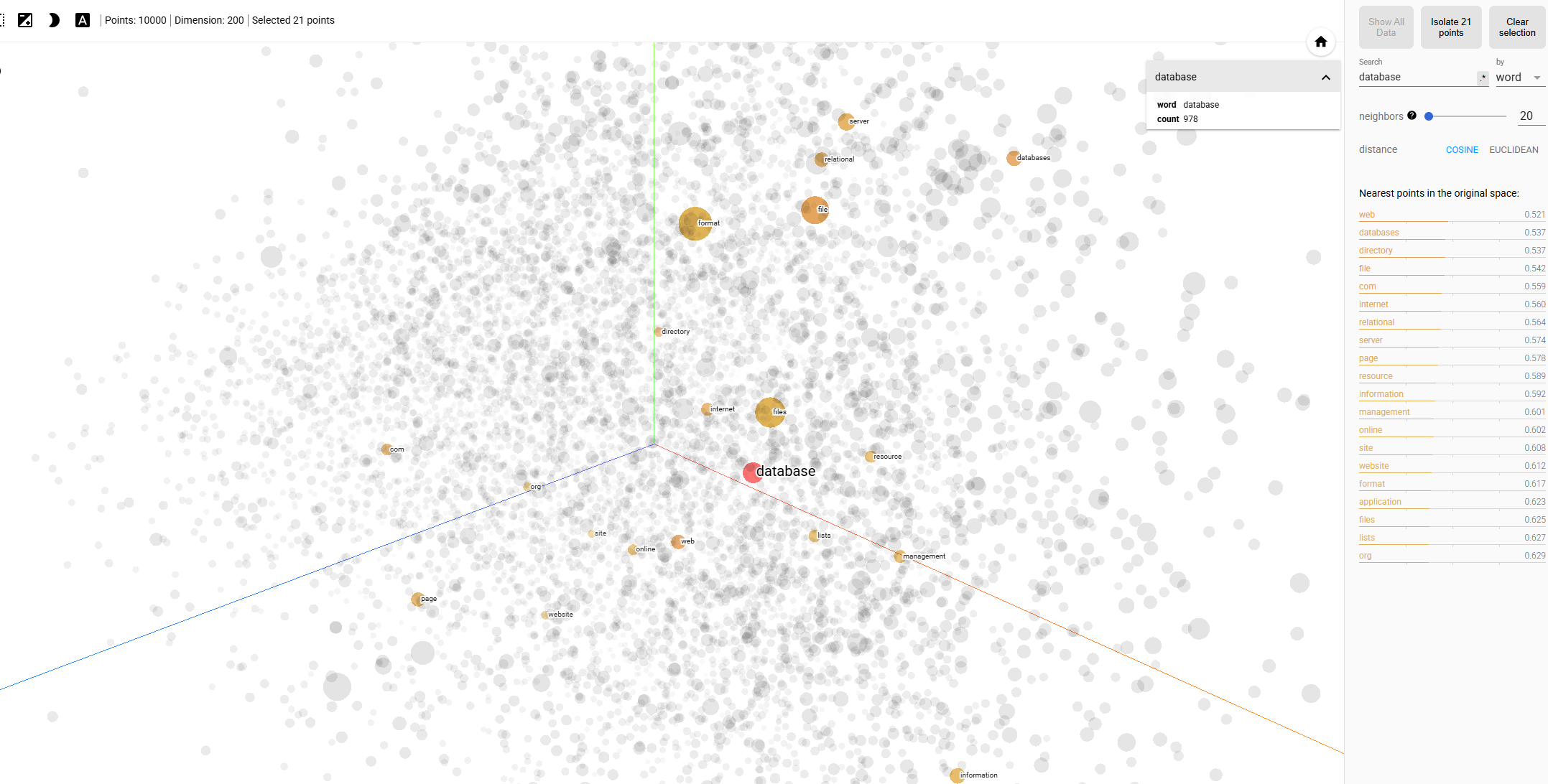
If embeddings are still a bit hard to understand you might want to check this visualization of vector embeddings through this URL :
Embedding projector – visualization of high-dimensional data
That’s it for now. In the coming part 3 of this series we will talk about AI agents and workflows and how they relate to a DBA. For the part 4 we will discuss AI workflows Best practices. We will see if there is a need for a part 5.
Referenced links :
pgvector/pgvector: Open-source vector similarity search for Postgres
DiskANN Vector Index in Azure Database for PostgreSQL
microsoft/DiskANN: Graph-structured Indices for Scalable, Fast, Fresh and Filtered Approximate Nearest Neighbor Search
timescale/pgvectorscale: A complement to pgvector for high performance, cost efficient vector search on large workloads.
Timescale Documentation | SQL inteface for pgvector and pgvectorscale
Debunking 6 common pgvector myths
Vector Indexes in Postgres using pgvector: IVFFlat vs HNSW | Tembo
Optimizing vector search performance with pgvector – Neon
![Thumbnail [60x60]](https://www.dbi-services.com/blog/wp-content/uploads/2025/03/OBA_web-scaled.jpg)