As the saying goes, “A Picture Is Worth A Thousands Words”. I’d add “And A Simple Graph Is Worth A Long, Abstruse List of Numbers”. And of words too, so let’s show off a little bit:
Interested ? Then, please read on.
It happens not so infrequently that we wish we could quickly plot a few numbers to have a look at their overall trend. The usual procedure is to output the numbers into a csv file, transfer it to a desktop machine, subsequently import it into a spreadsheet program and interactively set up a chart, a tedious manual procedure at best, especially if it has to be repeated several times.
What if we could query a few relevant values from a system and plot them in one go to visualize the produced graphs from within a browser ? What if we could generalize that procedure to any extracted tabular data ? I’m not talking of a sophisticated interface to some enterprise-class graphing tool but just of a simple way to get a quick visual overall feeling of some variables with as little installed software as possible.
I’ll show here how to do that for a Documentum repository but the target system can be anything, a database, an ldap, an O/S, just adapt the queries and the script as needed.
To simplify, I assume that we generally work on a server machine, likely a Linux headless VM, and that the browser runs remotely on any GUI-based desktop, quite a common configuration for Documentum.
The Data
As an administrator, I often have to connect to docbases I never visited before, and I find it useful to run the following queries to help me make acquaintance with those new beasts. In the examples below, the target docbase is an out of the box one with no activity in it, which explains the low numbers and lack of custom doctypes:
— 1. what distinct document types are there ?
select r_object_type, count(*), sum(r_full_content_size) as "tot_size" from dm_document(all) group by r_object_type order by 1

r_object_type                     count(*)                tot_size

--------------------------------  ----------------------  ----------------------

dm_document                                         1295                 6384130

dm_esign_template                                      1                   46255

dm_format_preferences                                  1                     109

dm_menu_system                                         2                  352034

dm_plugin                                              2                  212586

dm_xml_config                                          1                     534

dmc_jar                                              236                50451386

dmc_preset_package                                     2                   11951

dmc_tcf_activity_template                             10                   12162

(9 rows affected)
A reminder of some definitions: The result table above is a dataset. The r_object_type is the category, typically shown in the X-axis. The count(*) and tot_size columns are the “variables” to be plot, typically as bars, lines or pie slices. They are also named “traces” in some graphing tools. Some of the datasets here have 1, 2 or 3 variables to be plot. Datasets with 1 variable can be plot as bars, lines or pies charts. Datasets with 2 variables can be plot as grouped or stacked bars, or as 2 distinct graphs of one variable. There are many possibilities and combinations, and the choice depends on which representation offers the best visual clarity. Sometimes, the plotting library even lets one edit the programmatically generated graph and interactively choose the best type of graph with no coding needed !
— 2. how does their population vary over time ?
select r_object_type, datefloor(month, r_creation_date) as "creation_month", count(*), sum(r_full_content_size) as "tot_size" from dm_document(all) group by r_object_type, datefloor(month, r_creation_date) order by 1, 2;

r_object_type                     creation_month             count(*)      tot_size

--------------------------------  -------------------------  ------------  ------------

dm_document                       11/1/2017 01:00:00                  448       3055062

dm_document                       12/1/2017 01:00:00                  120        323552

dm_document                       3/1/2018 01:00:00                    38         66288

dm_document                       4/1/2018 02:00:00                   469       1427865

dm_document                       5/1/2018 02:00:00                    86        584453

dm_document                       6/1/2018 02:00:00                    20        150464

dm_document                       7/1/2018 02:00:00                    40        301341

dm_document                       8/1/2018 02:00:00                    32        151333

dm_document                       9/1/2018 02:00:00                    46        356386

dm_esign_template                 11/1/2017 01:00:00                    1         46255

dm_format_preferences             11/1/2017 01:00:00                    1           109

dm_menu_system                    11/1/2017 01:00:00                    2        352034

dm_plugin                         11/1/2017 01:00:00                    2        212586

dm_xml_config                     11/1/2017 01:00:00                    1           534

dmc_jar                           11/1/2017 01:00:00                  236      50451386

dmc_preset_package                11/1/2017 01:00:00                    2         11951

dmc_tcf_activity_template         11/1/2017 01:00:00                   10         12162

(17 rows affected)
This query tells how heavily used the repository is. Also, a broad spectre of custom document types tends to indicate that the repository is used in the context of applications.
— 3. how changing are those documents ?
select r_object_type, datefloor(month, r_modify_date) as "modification_month", count(*), sum(r_full_content_size) as "tot_size" from dm_document(all) where r_creation_date < r_modify_date group by r_object_type, datefloor(month, r_modify_date) order by 1, 2;

r_object_type                     modification_month         count(*)      tot_size

--------------------------------  -------------------------  ------------  ------------

dm_document                       11/1/2017 01:00:00                  127        485791

dm_document                       12/1/2017 01:00:00                   33        122863

dm_document                       3/1/2018 01:00:00                    16         34310

dm_document                       4/1/2018 02:00:00                   209        749370

dm_document                       5/1/2018 02:00:00                    42        311211

dm_document                       6/1/2018 02:00:00                    10         79803

dm_document                       7/1/2018 02:00:00                    20        160100

dm_document                       8/1/2018 02:00:00                    12         81982

dm_document                       9/1/2018 02:00:00                    23        172299

dm_esign_template                 8/1/2018 02:00:00                     1         46255

dmc_jar                           11/1/2017 01:00:00                   14       1616218

dmc_preset_package                11/1/2017 01:00:00                    2         11951

dmc_tcf_activity_template         11/1/2017 01:00:00                   10         12162

(13 rows affected)
This query shows if a repository is used interactively rather than for archiving. If there are lots of editions, the docbase is a lively one; on the contrary, if documents are rarely or never edited, the docbase is mostly used for archiving. The document ownership can tell too, technical accounts vs. real people.
— samething but without distinction of document type;
— 4. new documents;
select datefloor(month, r_creation_date) as "creation_month", count(*), sum(r_full_content_size) as "tot_size" from dm_document(all) group by datefloor(month, r_creation_date) order by 1;

creation_month             count(*)                tot_size

-------------------------  ----------------------  ----------------------

11/1/2017 01:00:00                            703                54142079

12/1/2017 01:00:00                            120                  323552

3/1/2018 01:00:00                              38                   66288

4/1/2018 02:00:00                             469                 1427865

5/1/2018 02:00:00                              86                  584453

6/1/2018 02:00:00                              20                  150464

7/1/2018 02:00:00                              40                  301341

8/1/2018 02:00:00                              32                  151333

9/1/2018 02:00:00                              42                  323772

(9 rows affected)
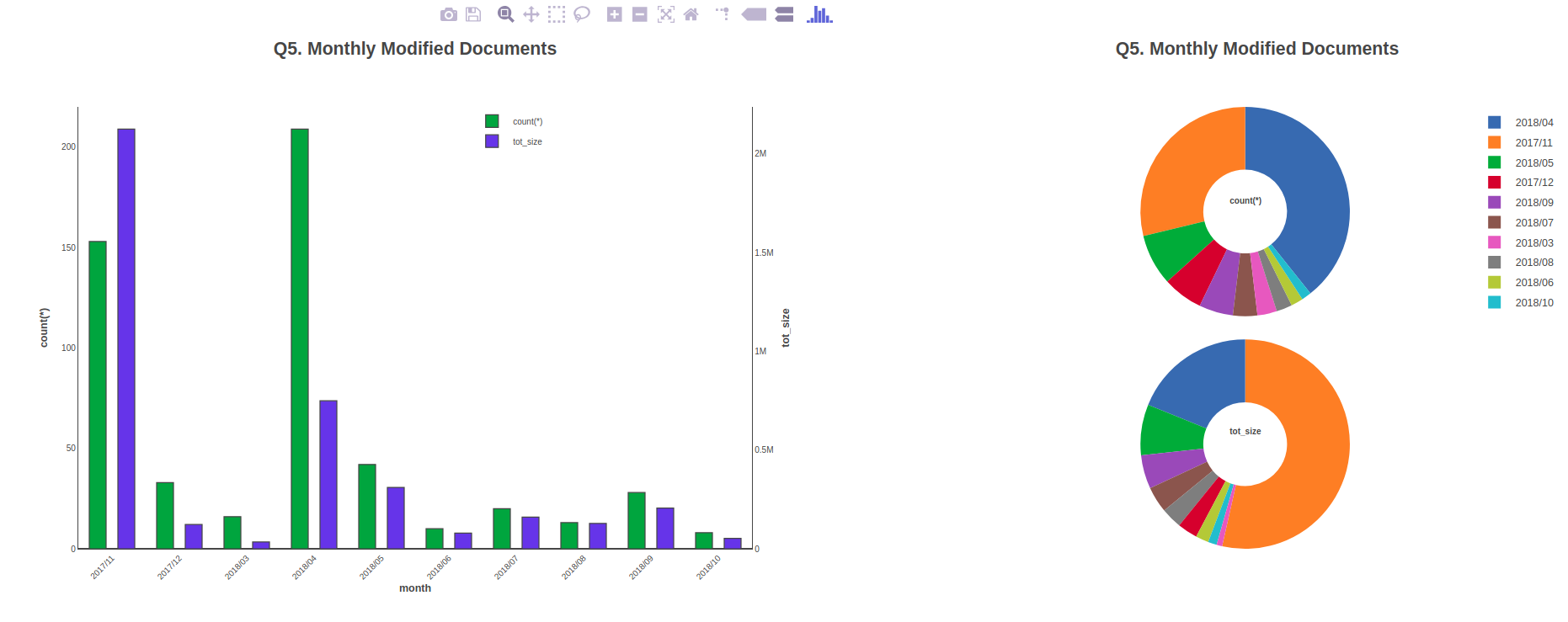
— 5. modified documents;
select datefloor(month, r_modify_date) as "modification_month", count(*), sum(r_full_content_size) as "tot_size" from dm_document(all) where r_creation_date < r_modify_date group by datefloor(month, r_modify_date) order by 1;

modification_month         count(*)                tot_size

-------------------------  ----------------------  ----------------------

11/1/2017 01:00:00                            153                 2126122

12/1/2017 01:00:00                             33                  122863

3/1/2018 01:00:00                              16                   34310

4/1/2018 02:00:00                             209                  749370

5/1/2018 02:00:00                              42                  311211

6/1/2018 02:00:00                              10                   79803

7/1/2018 02:00:00                              20                  160100

8/1/2018 02:00:00                              13                  128237

9/1/2018 02:00:00                              20                  140354

(9 rows affected)
— 6. what content types are used in the repository ?
select a_content_type, count(*) as "count_content_type", sum(r_full_content_size) as "tot_content_size" from dm_document(all) group by a_content_type order by 1

col a_content_type 20

a_content_type        count_content_type  tot_content_size

--------------------  ------------------  ----------------

                                      11                 0

amipro                                 1              4558

crtext                                43            389681

dtd                                    5            163392

excel12bbook                           1              8546

excel12book                            1              7848

excel12mebook                          1              7867

excel12metemplate                      1              7871

excel12template                        1              7853

excel5book                             1             15360

excel8book                             1             13824

excel8template                         1             13824

ibmshrlib                              2            212586

jar                                  233          48856783

java                                   3           1594603

maker55                                5            117760

mdoc55                                 9            780288

ms_access7                             1             83968

ms_access8                             1             59392

ms_access8_mde                         1             61440

msw12                                  1             11280

msw12me                                1             10009

msw12metemplate                        1             10004

msw12template                          1              9993

msw6                                   1             11776

msw8                                   1             19456

msw8template                           1             27136

pdf                                    2             50214

powerpoint                             1             14848

ppt12                                  1             29956

ppt12me                                1             29944

ppt12meslideshow                       1             29943

ppt12metemplate                        1             29941

ppt12slideshow                         1             29897

ppt12template                          1             29914

ppt8                                   1              7680

ppt8_template                          1              9728

text                                1175           4236008

ustn                                   1             10240

vrf                                    1            158993

wp6                                    1               941

wp7                                    1              1362

wp8                                    1              1362

xml                                   28             37953

zip                                    1            255125

(45 rows affected)
The content type may indicates the kind of activity the repository is used for. While pdf are generally final documents suitable for archiving, a predominance of illustrator/pagemaker/QuarkXPress vs photoshop vs multimedia vs Office documents can give a hint at the docbase’s general function.
Since most content types are unused (who uses Word Perfect or Ami Pro any more ?), a constraint on the count can be introduced, e.g. “having count(*) > 10” to filter out those obsolete formats.
— 7. and how do they evolve over time ?
select datefloor(month, r_creation_date) as "creation_month", a_content_type, count(*), sum(r_full_content_size) as "tot_size" from dm_document(all) group by datefloor(month, r_creation_date), a_content_type order by 1, 2

creation_month             a_content_type        count(*)      tot_size

-------------------------  --------------------  ------------  ------------

11/1/2017 01:00:00                                          1             0

11/1/2017 01:00:00         amipro                           1          4558

11/1/2017 01:00:00         crtext                          43        389681

11/1/2017 01:00:00         dtd                              5        163392

11/1/2017 01:00:00         excel12bbook                     1          8546

11/1/2017 01:00:00         excel12book                      1          7848

11/1/2017 01:00:00         excel12mebook                    1          7867

11/1/2017 01:00:00         excel12metemplate                1          7871

11/1/2017 01:00:00         excel12template                  1          7853

11/1/2017 01:00:00         excel5book                       1         15360

11/1/2017 01:00:00         excel8book                       1         13824

11/1/2017 01:00:00         excel8template                   1         13824

11/1/2017 01:00:00         ibmshrlib                        2        212586

11/1/2017 01:00:00         jar                            233      48856783

11/1/2017 01:00:00         java                             3       1594603

11/1/2017 01:00:00         maker55                          5        117760

11/1/2017 01:00:00         mdoc55                           9        780288

11/1/2017 01:00:00         ms_access7                       1         83968

11/1/2017 01:00:00         ms_access8                       1         59392

11/1/2017 01:00:00         ms_access8_mde                   1         61440

11/1/2017 01:00:00         msw12                            1         11280

11/1/2017 01:00:00         msw12me                          1         10009

11/1/2017 01:00:00         msw12metemplate                  1         10004

11/1/2017 01:00:00         msw12template                    1          9993

11/1/2017 01:00:00         msw6                             1         11776

11/1/2017 01:00:00         msw8                             1         19456

11/1/2017 01:00:00         msw8template                     1         27136

11/1/2017 01:00:00         pdf                              2         50214

11/1/2017 01:00:00         powerpoint                       1         14848

11/1/2017 01:00:00         ppt12                            1         29956

11/1/2017 01:00:00         ppt12me                          1         29944

11/1/2017 01:00:00         ppt12meslideshow                 1         29943

11/1/2017 01:00:00         ppt12metemplate                  1         29941

11/1/2017 01:00:00         ppt12slideshow                   1         29897

11/1/2017 01:00:00         ppt12template                    1         29914

11/1/2017 01:00:00         ppt8                             1          7680

11/1/2017 01:00:00         ppt8_template                    1          9728

11/1/2017 01:00:00         text                           338        906940

11/1/2017 01:00:00         ustn                             1         10240

11/1/2017 01:00:00         vrf                              1        158993

11/1/2017 01:00:00         wp6                              1           941

11/1/2017 01:00:00         wp7                              1          1362

11/1/2017 01:00:00         wp8                              1          1362

11/1/2017 01:00:00         xml                             28         37953

11/1/2017 01:00:00         zip                              1        255125

12/1/2017 01:00:00         text                           120        323552

3/1/2018 01:00:00          text                            38         66288

4/1/2018 02:00:00          text                           469       1427865

5/1/2018 02:00:00          text                            86        584453

6/1/2018 02:00:00          text                            20        150464

7/1/2018 02:00:00          text                            40        301341

8/1/2018 02:00:00                                          10             0

8/1/2018 02:00:00          text                            22        151333

9/1/2018 02:00:00          text                            42        323772

(54 rows affected)
— 8. where are those contents stored ?
select a_storage_type, count(*), sum(r_full_content_size) as "tot_size" from dm_document(all) group by a_storage_type order by a_storage_type

col a_storage_type 20

a_storage_type        count(*)      tot_size

--------------------  ------------  ------------

                                11             0

filestore_01                  1539      57471147

(2 rows affected)
Filestores are conceptually quite similar to Oracle RDBMS tablespaces. It is a good practice to separate filestores by applications/type of documents and/or even by time if the volume of documents in important. This query tells if this is in place and, if so, what the criteria were.
— 9. dig by document type;
select r_object_type, a_storage_type, count(*), sum(r_full_content_size) as "tot_size" from dm_document(all) group by r_object_type, a_storage_type order by r_object_type, a_storage_type

r_object_type                     a_storage_type        count(*)      tot_size

--------------------------------  --------------------  ------------  ------------

dm_document                                                       11             0

dm_document                       filestore_01                  1284       6384130

dm_esign_template                 filestore_01                     1         46255

dm_format_preferences             filestore_01                     1           109

dm_menu_system                    filestore_01                     2        352034

dm_plugin                         filestore_01                     2        212586

dm_xml_config                     filestore_01                     1           534

dmc_jar                           filestore_01                   236      50451386

dmc_preset_package                filestore_01                     2         11951

dmc_tcf_activity_template         filestore_01                    10         12162

(10 rows affected)
— 10. same but by content format;
select a_content_type, a_storage_type, count(*), sum(r_full_content_size) as "tot_size" from dm_document(all) group by a_content_type, a_storage_type having count(*) > 10 order by a_content_type, a_storage_type

a_content_type                    a_storage_type   count(*)                tot_size

--------------------------------  ---------------  ----------------------  ----------------------

crtext                            filestore_01                         43                  389681

jar                               filestore_01                        233                48856783

text                              filestore_01                       1204                 4432200

xml                               filestore_01                         28                   37953

(4 rows affected)
— 11. what ACLs do exist and who created them ?
select owner_name, count(*) from dm_acl group by owner_name order by 2 desc

col owner_name 30

owner_name                      count(*)

------------------------------  ------------

dmadmin                                  179

dmtest                                    44

dm_bof_registry                            6

dmc_wdk_preferences_owner                  2

dmc_wdk_presets_owner                      2

dm_mediaserver                             1

dm_audit_user                              1

dm_autorender_mac                          1

dm_fulltext_index_user                     1

dm_autorender_win31                        1

dm_report_user                             1

(11 rows affected)
Spoiler alert: the attentive readers have probably noticed the command “col” preceding several queries, like in “col name 20”; this is not a standard idql command but part of an extended idql which will be presented in a future blog.
ACLs are part of the security model in place, if any. Usually, the owner is a technical account, sometimes a different one for each application or application’s functionality or business line, so this query can show if the repository is under control of applications or rather simply used as a replacement for a shared drive. Globally, it can tell how the repository’s security is managed, if at all.
— 12. ACLs most in use;
select acl_name, count(*) from dm_document(all) where acl_name not like 'dm_%' group by acl_name having count(*) >= 10 order by 1

acl_name                          count(*)

--------------------------------  ----------------------

BOF_acl                                              233

(1 row affected)
Here too, a filter by usage can be introduced so that rarely used acls are not reported, e.g. “having count(*) > 10”.
— 13. queue items;
select name, count(*) from dmi_queue_item group by name order by 2 desc

name                  count(*)

--------------------  ------------

dm_autorender_win31            115

dmadmin                        101

dmtest                          54

(3 rows affected)
This query is mainly useful to show if external systems are used for generating renditions, thumbnails or any other document transformation.
— non quantifiable queries;
select object_name from dm_acl where object_name not like 'dm_%' order by 1

object_name

--------------------------------

BOF_acl

BOF_acl2

BPM Process Variable ACL

BatchPromoteAcl

Default Preset Permission Set

Global User Default ACL

WebPublishingAcl

Work Queue User Default ACL

dce_world_write

desktop_client_acl1

replica_acl_default

(11 rows affected)


col name 20

col root 30

col file_system_path 70

select f.name, f.root, l.file_system_path from dm_filestore f, dm_location l where f.root = l.object_name

name                  root                            file_system_path

--------------------  ------------------------------  ----------------------------------------------------------------------

filestore_01          storage_01                      /home/dmadmin/documentum/data/dmtest/content_storage_01

thumbnail_store_01    thumbnail_storage_01            /home/dmadmin/documentum/data/dmtest/thumbnail_storage_01

streaming_store_01    streaming_storage_01            /home/dmadmin/documentum/data/dmtest/streaming_storage_01

replicate_temp_store  replicate_location              /home/dmadmin/documentum/data/dmtest/replicate_temp_store

replica_filestore_01  replica_storage_01              /home/dmadmin/documentum/data/dmtest/replica_content_storage_01

(5 rows affected)
No numbers here, just plain text information.
There is of course much more information to query (e.g. what about lifecycles and workflows, users and groups ?) depending on what one needs to look at in the repositories, but those are enough examples for our demonstration’s purpose. The readers can always add queries or refine the existing ones to suit their needs.
At this point, we have a lot of hard-to-ingest numbers. Plotting them gives a pleasant 2-dimensional view of the data and will allow to easily compare and analyze them, especially if the generated plot offers some interactivity.
The Graphing Library
To do this, we need a graphing library and since we want to be able to look at the graphs from within a browser for platform-independence and zero-installation on the desktop, we need one that lets us generate an HTML page containing the charts. This is possible in 2 ways:
o the library is a javascript one; we will programmatically build up json literals, pass them to the library’s plotting function and wrap everything into an html page which is saved on disk for later viewing;
o the library is usable from several scripting languages and includes a function to generate an HTML page containing the graph; we will chose one for python since this language is ubiquitous and we have now a binding for Documentum (see my blog here);
Now, there are tons of such javascript libraries available on-line (see for example here for a sample) but our choice criteria will be simple:
o the library must be rich enough but at the same time easy to use;
o it must do its work entirely locally as servers are generally not allowed to access the Internet;
o it must be free in order to get rid of the licensing complexity as it can often be overkill in such a simple and confined usage;
As we must pick one, let’s choose Plotly since it is very capable and largely covers our needs. Besides, it works either as a javascript or as a python library but for more generality let’s just use it as a javascript library and generate ourselves the html pages. As an additional bonus, Plotly also allows to interactively edit a plotted graph so it can be tweaked at will. This is very convenient because it lessens the effort to optimize the graphs’ readability as this can be done later by the users themselves while viewing the graphs. For example, the users can zoom, unselect variables, move legends around and much more.
To install it, simply right-click here and save the link to the default graph location in the project’s directory, e.g. /home/dmadmin/graph-stats/graphs.
pwd

/home/dmadmin/graph-stats/graphs

ls -l

...

-rw-rw-r-- 1 dmadmin dmadmin 2814564 Oct 11 11:40 plotly-latest.min.js

...
That’s less than 2.7 MiB of powerful compact js source code. Since it is a text file, there shouldn’t be any security concern in copying that file on a server. Also, as it is executed inside the sandbox of a browser, security is normally not an issue.
The library needs to be in the same directory as the generated html files. If those files are copied to a desktop for direct viewing from a browser with File/Open, don’t forget to copy over the Plotly.js library too, open the html file in an editor, go to the line 6 below and set src to the path of the html file:
<!DOCTYPE html PUBLIC "-//W3C//DTD HTML 3.2//EN">
<html>
   <head>
      <title>Graphical Overview of Repository SubWay</title>
      <meta http-equiv="Content-Type" content="text/html; charset=utf-8">
      <script src="...../plotly-latest.min.js"></script>
   </head>
Viewing the html pages
Since those pages must be accessed from any machine on the network (typically, a desktop with a browser), despite they may be created directly on the server that hosts the repositories of interest, we need a web server. It may happen that a disk volume is shared between desktops and servers but this is far from being the general case. Fortunately, python is very helpful here and saves us from the tedious task of setting up a full-fledged web server such as apache. The one-liner below will start a server for visualizing the files in the current directory and its sub-directories:
python3 -m http.server [port]     # for python >= v3

python -m SimpleHTTPServer [port] # for python 2.x
It can also be moved in the background to free the command-line. To stop it, bring it in the foreground and type ctrl-C.
Its default port is 8000.
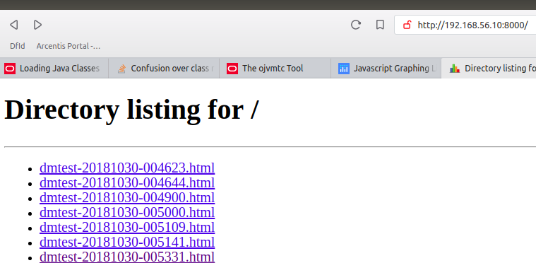
This mini-web server is now waiting for requests on the given port and its IP address. In order to determine that IP address, use the ifconfig command and try one address that is on the same network as the desktop with the browser. Then, load the URL, e.g. http://192.168.56.10:8000/, and you’ll be greeted by a familiar point-and-click interface.
The server presents a directory listing from which to select the html files containing the generated graphs.
An Example
Here is a complete example, from the query to the graph.
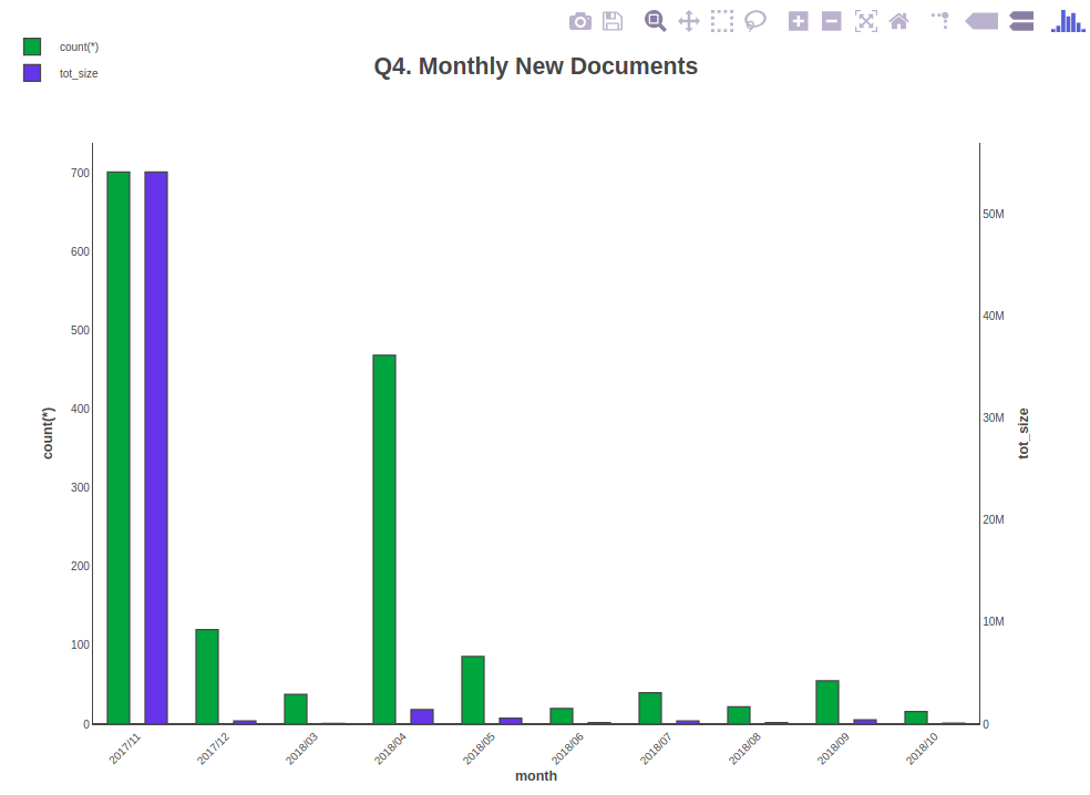
The 4th DQL query and its output:
select datefloor(month, r_creation_date) as "creation_month", count(*), sum(r_full_content_size) as "tot_size" from dm_document(all) group by datefloor(month, r_creation_date) order by 1;

creation_month             count(*)                tot_size

-------------------------  ----------------------  ----------------------

11/1/2017 01:00:00                            703                54142079

12/1/2017 01:00:00                            120                  323552

3/1/2018 01:00:00                              38                   66288

4/1/2018 02:00:00                             469                 1427865

5/1/2018 02:00:00                              86                  584453

6/1/2018 02:00:00                              20                  150464

7/1/2018 02:00:00                              40                  301341

8/1/2018 02:00:00                              32                  151333

9/1/2018 02:00:00                              42                  323772

(9 rows affected)
The command to generate the graph:
pwd

/home/dmadmin/graph-stats

./graph-stats.py --docbase dmtest
A simplified generated html page showing only the count(*) variable:
<!DOCTYPE html PUBLIC "-//W3C//DTD HTML 3.2//EN">
<html>
      <head>
         <title>Statistical Graphs for Repository dmtest</title>
         <meta http-equiv="Content-Type" content="text/html; charset=utf-8">
         <script src="http://192.168.56.10:8000/plotly-latest.min.js"></script>
      </head>
      <body>
      <div id="TheChart" style="width:400px;height:400px;"></div>
      <script>
         var ctx = document.getElementById("TheChart");
         Plotly.newPlot(ctx, [{
                             type: "bar",
                             name: "new docs",
                             x: ['2017/11', '2017/12', '2018/03', '2018/04', '2018/05', '2018/06', '2018/07', '2018/08', '2018/09'],
                             y: ['703', '120', '38', '469', '86', '20', '40', '32', '42'],
                             marker: {
                                        color: '#4e6bed',
                                        line: {
                                                 width: 2.5
                                              }
                                     }
                            }],
                            {
                               title: "New Documents",
                               font: {size: 18}
                            },
                        {responsive: true});
      </script>
      </body>
</html>
Its resulting file:
ll graphs

total 2756

-rw-rw-r-- 1 dmadmin dmadmin 2814564 Oct 12 14:18 plotly-latest.min.js

-rw-rw-r-- 1 dmadmin dmadmin    1713 Oct 12 14:18 dmtest-20181012-141811.html
Same but exposed by the mini-web server and viewed from a browser:
When clicking on one of the html file, a graph such as the one below is displayed:
The python script
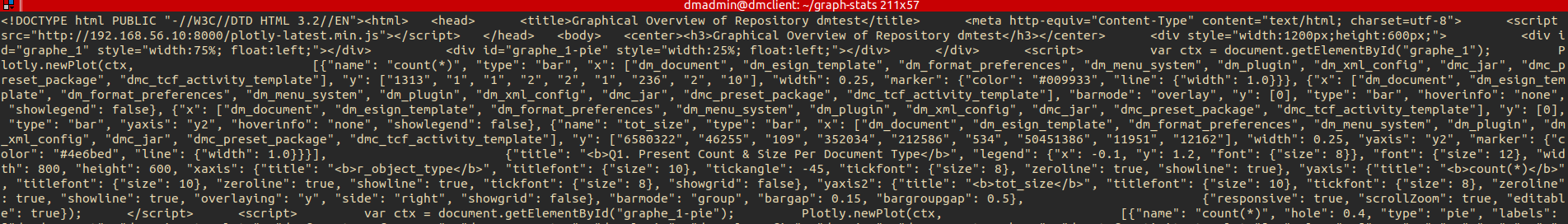
The following python script runs the 13 queries above and produce one large HTML page containing the graphs of all the datasets. It can also be used to query a list of local docbases and generate one single, huge html report or one report per docbase. It can even directly output the produced html code to stdout for further in-line processing, e.g. to somewhat compact the javascript code:
./graph-stats.py --docbase dmtest -o stdout | gawk '{printf $0}' > graphs/dmtest-gibberish.html


wc -l graphs/-gibberish.html

0 graphs/-gibberish.html


less graphs/dmtest-gibberish.html
So, here is the script:
#!/usr/bin/env python
# 10/2018, C. Cervini, dbi-services;
import sys
import getopt
from datetime import datetime
import json
import DctmAPI
def Usage():
print("""
Usage:
Connects as dmadmin/xxxx to a local repository and generates an HTML page containing the plots of several DQL queries result;
Usage:
./graph-stats.py -h|--help | -d|--docbase <docbase>{,<docbase>} \[-o|--output_file <output_file>\]
<docbase> can be one repository or a comma-separated list of repositories;
if <output_file> is omitted, the html page is output to ./graphs/<docbase>-$(date +"%Y%m%d-%H%M%S").html;
<output_file> can be "stdout", which is useful for CGI programming;
Example:
./graph-stats.py -d dmtest,mail_archive,doc_engineering
will query the docbases dmtest, mail_archive and doc_engineering and output the graphs to the files <docbase>-$(date +"%Y%m%d-%H%M%S").html, one file per docbase;
./graph-stats.py -d mail_archive,doc_engineering -o all_docbase_current_status
will query the docbases mail_archive and doc_engineering and output all the graphs to the unique file all_docbase_current_status;
./graph-stats.py -d mail-archive
will query docbase mail-archive and output the graphs to the file mail-archive-$(date +"%Y%m%d-%H%M%S").html;
./graph-stats.py --docbase dmtest --output dmtest.html
will query docbase dmtest and output the graphs to the file dmtest.html;
./graph-stats.py -d dmtest --output stdout
will query docbase dmtest and output the graphs to stdout;
""")
def Plot2HTML(div, graph_title, data, data_labels, bLineGraph = False, mode = None):
global html_output
if None != html_output:
sys.stdout = open(html_output, "a")
# start the html page;
if "b" == mode:
global server, page_title
print('''
<!DOCTYPE html PUBLIC "-//W3C//DTD HTML 3.2//EN">
<html>
<head>
<title>''' + page_title + '''</title>
<meta http-equiv="Content-Type" content="text/html; charset=utf-8">
<script src="http://''' + server + '''/plotly-latest.min.js"></script>
</head>
<body>
<center><h3>''' + page_title + '''</h3></center>
''')
# append to the body of the html page;
if len(data_labels) == 4:
stack_labels = {}
for point in data:
stack_labels[point[data_labels[0]]] = 0
print('''
<div style="width:1500px;height:600px;">
<div id="''' + div + '-' + data_labels[2] + '''" style="width:50%; float:left;"></div>
<div id="''' + div + '-' + data_labels[3] + '''" style="width:50%; float:left;"></div>
</div>
<script>
var ctx = document.getElementById("''' + div + '-' + data_labels[2] + '''");
''')
variables = ""
for stack in stack_labels:
x = [point[data_labels[1]] for i, point in enumerate(data) if point[data_labels[0]] == stack]
y1 = [point[data_labels[2]] for i, point in enumerate(data) if point[data_labels[0]] == stack]
variables += ("" if not variables else ", ") + "data_" + stack
if bLineGraph:
vars()['data_' + stack] = {
'name': stack,
'type': "scatter",
'mode': "lines",
'x': x,
'y': y1,
};
else:
vars()['data_' + stack] = {
'name': stack,
'type': "bar",
'x': x,
'y': y1,
'width': 0.25,
'marker': {
#'color': '#009933',
'line': {
'width': 1.0
}
}
};
print('data_' + stack + ' = ' + json.dumps(vars()['data_' + stack]) + ';')
layout = {
'title': '<b>' + graph_title + '<br>' + data_labels[2] + '</b>',
'legend': {'x': -.1, 'y': 1.2, 'font': {'size': 8}},
'font': {'size': 12},
'width': 750,
'height': 600,
'xaxis': {
'title': '<b>' + data_labels[1] + '</b>',
'titlefont': {'size': 10},
'tickangle': -45,
'tickfont': {'size': 8},
'zeroline': True,
'showline': True,
'categoryorder': "category ascending",
'type': "category"
},
'yaxis': {
'title': '<b>' + data_labels[2] + '</b>',
'titlefont': {'size': 10},
'zeroline': True,
'showline': True,
'tickfont': {'size': 8},
'showgrid': False
}
}
if not bLineGraph:
layout.update({'barmode': "stack", 'bargap': 0.15, 'bargroupgap': 0.5})
interaction = {'responsive': True, 'scrollZoom': True, 'editable': True}
print('''Plotly.newPlot(ctx,
[''' + variables + '], ' +
json.dumps(layout) + ',' +
json.dumps(interaction) + ''');''')
for stack in stack_labels:
x = [point[data_labels[1]] for i, point in enumerate(data) if point[data_labels[0]] == stack]
y2 = [point[data_labels[3]] for i, point in enumerate(data) if point[data_labels[0]] == stack]
if bLineGraph:
vars()['data_' + stack] = {
'name': stack,
'type': "scatter",
'mode': "lines",
'x': x,
'y': y2
};
else:
vars()['data_' + stack] = {
'name': stack,
'type': "bar",
'x': x,
'y': y2,
'width': 0.25,
'marker': {
#'color': '#009933',*/
'line': {
'width': 1.0
}
}
};
print('data_' + stack + ' = ' + json.dumps(vars()['data_' + stack]) + ';')
layout = {
'title': '<b>' + graph_title + '<br>' + data_labels[3] + '</b>',
'legend': {'x': -.1, 'y': 1.2, 'font': {'size': 8}},
'font': {
'size': 12
},
'width': 750,
'height': 600,
'xaxis': {
'title': '<b>' + data_labels[1] + '</b>',
'titlefont': {'size': 10},
'tickangle': -45,
'tickfont': {'size': 8},
'zeroline': True,
'showline': True,
'categoryorder': "category ascending",
'type': "category"
},
'yaxis': {
'title': '<b>' + data_labels[3] + '</b>',
'titlefont': {'size': 10},
'zeroline': True,
'showline': True,
'tickfont': {'size': 8},
'showgrid': False
}
}
if not bLineGraph:
layout.update({'barmode': "stack", 'bargap': 0.15, 'bargroupgap': 0.5})
interaction = {'responsive': True, 'scrollZoom': True, 'editable': True}
print('''
var ctx = document.getElementById("''' + div + '-' + data_labels[3] + '''");
Plotly.newPlot(ctx,
[''' + variables + '],' +
json.dumps(layout) + ''',
''' + json.dumps(interaction) + ''');
</script>
''')
elif len(data_labels) == 3:
print('''
<div style="width:1200px;height:600px;">
<div id="''' + div + '''" style="width:75%; float:left;"></div>
<div id="''' + div + '''-pie" style="width:25%; float:left;"></div>
</div>
<script>
var ctx = document.getElementById("''' + div + '''");
''')
traces = []
if not bLineGraph:
traces = [
{
'name': data_labels[1],
'type': "bar",
'x': [point[data_labels[0]] for i, point in enumerate(data)],
'y': [point[data_labels[1]] for i, point in enumerate(data)],
'width': 0.25,
'marker': {
'color': '#009933',
'line': {
'width': 1.0
}
},
},
# work around for bug "Grouped bar charts do not work with multiple Y axes";
# see https://github.com/plotly/plotly.js/issues/78;
# must be inserted here;
# invisible second trace in the first group
{
'x': [point[data_labels[0]] for i, point in enumerate(data)],
'barmode': "overlay",
'y': [0], 'type': 'bar', 'hoverinfo': 'none', 'showlegend': False
},
# invisible first trace in the second group
{
'x': [point[data_labels[0]] for i, point in enumerate(data)],
'y': [0], 'type': 'bar', 'yaxis': 'y2', 'hoverinfo': 'none', 'showlegend': False
},
{
'name': data_labels[2],
'type': "bar",
'x': [point[data_labels[0]] for i, point in enumerate(data)],
'y': [point[data_labels[2]] for i, point in enumerate(data)],
'width': 0.25,
'yaxis': "y2",
'marker': {
'color': '#4e6bed',
'line': {
'width': 1.0
}
}
}
]
else:
traces = [
{
'name': data_labels[1],
'type': "scatter",
'mode': "lines",
'x': [point[data_labels[0]] for i, point in enumerate(data)],
'y': [point[data_labels[1]] for i, point in enumerate(data)],
'width': 0.25,
},
{
'name': data_labels[2],
'type': "scatter",
'mode': "lines",
'x': [point[data_labels[0]] for i, point in enumerate(data)],
'y': [point[data_labels[2]] for i, point in enumerate(data)],
'width': 0.25,
'yaxis': "y2",
}
]
layout = {
'title': '<b>' + graph_title + '</b>',
'legend': {'x': -.1, 'y': 1.2, 'font': {'size': 8}},
'font': {'size': 12},
'width': 800,
'height': 600,
'xaxis': {
'title': '<b>' + data_labels[0] + '</b>',
'titlefont': {'size': 10},
'tickangle': -45,
'tickfont': {'size': 8},
'zeroline': True,
'showline': True
},
'yaxis': {
'title': '<b>' + data_labels[1] + '</b>',
'titlefont': {'size': 10},
'zeroline': True,
'showline': True,
'tickfont': {'size': 8},
'showgrid': False,
},
'yaxis2': {
'title': '<b>' + data_labels[2] + '</b>',
'titlefont': {'size': 10},
'tickfont': {'size': 8},
'zeroline': True,
'showline': True,
'overlaying': "y",
'side': "right",
'showgrid': False,
}
}
if bLineGraph:
layout['yaxis'].update({'type': "linear"})
layout['yaxis2'].update({'type': "linear"})
pass
else:
layout.update({'barmode': "group", 'bargap': 0.15, 'bargroupgap': 0.5})
interaction = {'responsive': True, 'scrollZoom': True, 'editable': True}
print('''
Plotly.newPlot(ctx,
''' + json.dumps(traces) + ''',
''' + json.dumps(layout) + ''',
''' + json.dumps(interaction) + ''');
</script>
''')
if not bLineGraph:
traces = [
{
'name': data_labels[1],
'hole': .4,
'type': "pie",
'labels': [point[data_labels[0]] for i, point in enumerate(data)],
'values': [point[data_labels[1]] for i, point in enumerate(data)],
'domain': {
'row': 0,
'column': 0
},
'outsidetextfont': {'size': 8},
'insidetextfont': {'size': 8},
'legend': {'font': {'size': 8}},
'textfont': {'size': 8},
'font': {'size': 8},
'hoverinfo': 'label+percent+name',
'hoverlabel': {'font': {'size': 8}},
'textinfo': 'none'
},
{
'name': data_labels[2],
'hole': .4,
'type': "pie",
'labels': [point[data_labels[0]] for i, point in enumerate(data)],
'values': [point[data_labels[2]] for i, point in enumerate(data)],
'domain': {
'row': 1,
'column': 0
},
'outsidetextfont': {'size': 8},
'insidetextfont': {'size': 8},
'legend': {'font': {'size': 8}},
'textfont': {'size': 8},
'font': {'size': 8},
'hoverinfo': 'label+percent+name',
'hoverlabel': {'font': {'size': 8}},
'textinfo': 'none'
},
]
layout = {
'title': '<b>' + graph_title + '</b>',
'annotations': [
{
'font': {
'size': 8
},
'showarrow': False,
'text': '<b>' + data_labels[1] + '</b>',
'x': 0.5,
'y': 0.8
},
{
'font': {
'size': 8
},
'showarrow': False,
'text': '<b>' + data_labels[2] + '</b>',
'x': 0.5,
'y': 0.25
}
],
'height': 600,
'width': 600,
'grid': {'rows': 2, 'columns': 1},
'legend': {'font': {'size': 10}}
}
print('''
<script>
var ctx = document.getElementById("''' + div + '''-pie");
Plotly.newPlot(ctx,
''' + json.dumps(traces) + ''',
''' + json.dumps(layout) + '''
);
</script>
''')
elif len(data_labels) == 2:
trace = [
{
'name': data_labels[1],
'type': "bar",
'x': [point[data_labels[0]] for i, point in enumerate(data)],
'y': [point[data_labels[1]] for i, point in enumerate(data)],
'width': 0.25,
'marker': {
'color': '#009933',
'line': {
'width': 1.0
}
}
}
]
layout = {
'title': '<b>' + graph_title + '</b>',
'legend': {'x': -.1, 'y': 1.2, 'font': {'size': 8}},
'font': {'size': 12},
'height': 600,
'width': 800,
'xaxis': {
'title': '<b>' + data_labels[0] + '</b>',
'titlefont': {'size': 10},
'tickangle': -45,
'tickfont': {'size': 8},
'zeroline': True,
},
'yaxis': {
'title': '<b>' + data_labels[1] + '</b>',
'titlefont': {'size': 10},
'zeroline': True,
'showline': True,
'tickfont': {'size': 8},
'showgrid': False
},
'barmode': "group",
'bargap': 0.15,
'bargroupgap': 0.5
}
interaction = {'responsive': True, 'scrollZoom': True, 'editable': True};
print('''
<div style="width:1200px;height:600px;">
<div id="''' + div + '''" style="width:75%; float:left;"></div>
<div id="''' + div + '''-pie" style="width:25%; float:left;"></div>
</div>
<script>
var ctx = document.getElementById("''' + div + '''");
Plotly.newPlot(ctx,
''' + json.dumps(trace) + ''',
''' + json.dumps(layout) + ''',
''' + json.dumps(interaction) + ''');
</script>
''')
trace = [
{
'name': data_labels[1],
'hole': .4,
'type': "pie",
'labels': [point[data_labels[0]] for i, point in enumerate(data)],
'values': [point[data_labels[1]] for i, point in enumerate(data)],
'domain': {
'row': 0,
'column': 0
},
'outsidetextfont': {'size': 8},
'insidetextfont': {'size': 8},
'legend': {'font': {'size': 8}},
'textfont': {'size': 8},
'font': {'size': 8},
'hoverinfo': 'label+percent+name',
'hoverlabel': {'font': {'size': 8}},
'textinfo': 'none'
},
]
layout = {
'title': '<b>' + graph_title + '</b>',
'annotations': [
{
'font': {
'size': 8
},
'showarrow': False,
'text': '<b>' + data_labels[1] + '</b>',
'x': 0.5,
'y': 0.5
},
],
'height': 600,
'width': 600,
'grid': {'rows': 1, 'columns': 1},
'legend': {'font': {'size': 10}}
}
print('''
<script>
var ctx = document.getElementById("''' + div + '''-pie");
Plotly.newPlot(ctx,
''' + json.dumps(trace) + ''',
''' + json.dumps(layout) + ''');
</script>
''')
else:
print("illegal data_label value: " + repr(data_label))
# closes the html page;
if "e" == mode:
print('''
</body>
</html>
''')
# restores default output stream;
if None != html_output:
sys.stdout = sys.__stdout__
def cumulAndExtend2():
"""
for 2 variables in resultset;
"""
global rawdata
sum_count = 0
sum_size = 0
new_month = str(datetime.now().year) + "/" + str(datetime.now().month)
for ind, point in enumerate(rawdata):
sum_count += int(point['count(*)'])
point['count(*)'] = sum_count
sum_size += int(point['tot_size'])
point['tot_size'] = sum_size
if rawdata[ind]['month'] < new_month:
new_point = dict(rawdata[ind])
new_point['month'] = new_month
rawdata.append(new_point)
DctmAPI.show(rawdata)
def cumulAndExtend3(key):
"""
for 3 variables in resultset;
"""
global rawdata
prec_doc = ""
sum_count = 0
sum_size = 0
new_month = str(datetime.now().year) + "/" + str(datetime.now().month)
for ind, point in enumerate(rawdata):
if "" == prec_doc:
prec_doc = point[key]
if point[key] != prec_doc:
# duplicate the last point so the line graphe shows a flat line and not a simple dot when there is a unique point for the document type;
if rawdata[ind - 1]['month'] < new_month:
new_point = dict(rawdata[ind - 1])
new_point['month'] = new_month
rawdata.insert(ind, new_point)
prec_doc = point[key]
sum_count = 0
sum_size = 0
else:
sum_count += int(point['count(*)'])
point['count(*)'] = sum_count
sum_size += int(point['tot_size'])
point['tot_size'] = sum_size
if rawdata[ind]['month'] < new_month:
new_point = dict(rawdata[ind])
new_point['month'] = new_month
rawdata.append(new_point)
DctmAPI.show(rawdata)
# -----------------
# main;
if __name__ == "__main__":
DctmAPI.logLevel = 0
# parse the command-line parameters;
# old-style for I don't need more flexibility here;
repository = None
output_file = None
try:
(opts, args) = getopt.getopt(sys.argv[1:], "hd:o:", ["help", "docbase=", "output="])
except getopt.GetoptError:
print("Illegal option")
print("./graph-stats.py -h|--help | -d|--docbase <docbase>{,<docbase>} [-o|--output_file <output_file>]")
sys.exit(1)
for opt, arg in opts:
if opt in ("-h", "--help"):
Usage()
sys.exit()
elif opt in ("-d", "--docbase"):
repository = arg
elif opt in ("-o", "--output"):
output_file = arg
if None == repository:
print("at least one repository must be specified")
Usage()
sys.exit()
DctmAPI.show("Will connect to docbase(s): " + repository + " and output to " + ("stdout" if "stdout" == output_file else "one single file " + output_file if output_file is not None else "one file per docbase"))
# needed to locally import the js library Plotly;
server = "192.168.56.10:8000"
docbase_done = set()
status = DctmAPI.dmInit()
for pointer, docbase in enumerate(repository.split(",")):
# graphe_1;
if docbase in docbase_done:
print("Warning: docbase {:s} was already processed and won't be again, skipping ...".format(docbase))
continue
docbase_done.add(docbase)
session = DctmAPI.connect(docbase = docbase, user_name = "dmadmin", password = "dmadmin")
if session is None:
print("no session opened, exiting ...")
exit(1)
page_title = "Graphical Overview of Repository " + docbase
if None == output_file:
html_output = "./graphs/" + docbase + "-" + datetime.today().strftime("%Y%m%d-%H%M%S") + ".html"
elif "stdout" == output_file:
html_output = None
else:
html_output = output_file
graph_name = "graphe_1"
DctmAPI.show(graph_name, beg_sep = True)
stmt = """select r_object_type, count(*), sum(r_full_content_size) as "tot_size" from dm_document(all) group by r_object_type order by 1"""
rawdata = []
attr_name = []
status = DctmAPI.select2dict(session, stmt, rawdata, attr_name)
DctmAPI.show(rawdata)
if not status:
print("select [" + stmt + "] was not successful")
exit(1)
Plot2HTML(div = graph_name,
graph_title = "Q1. Present Count & Size Per Document Type",
data = rawdata,
data_labels = attr_name,
mode = ("b" if (("stdout" == output_file or output_file is not None) and 0 == pointer) or output_file is None else None))
# graphe_2;
graph_name = "graphe_2"
DctmAPI.show(graph_name, beg_sep = True)
stmt = """select r_object_type, datetostring(r_creation_date, 'yyyy/mm') as "month", count(*), sum(r_full_content_size) as "tot_size" from dm_document(all) group by r_object_type, datetostring(r_creation_date, 'yyyy/mm') order by 1, 2"""
rawdata = []
attr_name = []
status = DctmAPI.select2dict(session, stmt, rawdata, attr_name)
DctmAPI.show(rawdata)
if not status:
print("select [" + stmt + "] was not successful")
exit(1)
Plot2HTML(div = graph_name,
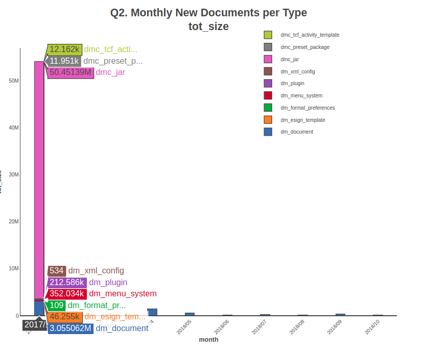
graph_title = "Q2. Monthly New Documents per Type",
data = rawdata,
data_labels = attr_name)
cumulAndExtend3('r_object_type')
Plot2HTML(div = graph_name + "l",
graph_title = "Q2l. Cumulated Monthly Documents per Type",
data = rawdata,
data_labels = attr_name,
bLineGraph = True)
# graphe_3;
graph_name = "graphe_3"
DctmAPI.show(graph_name, beg_sep = True)
stmt = """select r_object_type, datetostring(r_modify_date, 'yyyy/mm') as "month", count(*), sum(r_full_content_size) as "tot_size" from dm_document(all) where r_creation_date < r_modify_date group by r_object_type, datetostring(r_modify_date, 'yyyy/mm') order by 1, 2"""
rawdata = []
attr_name = []
status = DctmAPI.select2dict(session, stmt, rawdata, attr_name)
DctmAPI.show(rawdata)
if not status:
print("select [" + stmt + "] was not successful")
exit(1)
Plot2HTML(div = graph_name,
graph_title = "Q3. Monthly Modified Documents per Type",
data = rawdata,
data_labels = attr_name)
cumulAndExtend3('r_object_type')
Plot2HTML(div = graph_name + "l",
graph_title = "Q3l. Cumulated Monthly Modified Documents per Type",
data = rawdata,
data_labels = attr_name,
bLineGraph = True)
# graphe_4;
graph_name = "graphe_4"
DctmAPI.show(graph_name, beg_sep = True)
stmt = """select datetostring(r_creation_date, 'yyyy/mm') as "month", count(*), sum(r_full_content_size) as "tot_size" from dm_document(all) group by datetostring(r_creation_date, 'yyyy/mm') order by 1"""
rawdata = []
attr_name = []
status = DctmAPI.select2dict(session, stmt, rawdata, attr_name)
DctmAPI.show(rawdata)
if not status:
print("select [" + stmt + "] was not successful")
exit(1)
Plot2HTML(div = graph_name,
graph_title = "Q4. Monthly New Documents",
data = rawdata,
data_labels = attr_name )
cumulAndExtend2()
Plot2HTML(div = graph_name + "l",
graph_title = "Q4l. Cumulated Monthly Documents",
data = rawdata,
data_labels = attr_name,
bLineGraph = True)
# graphe_5;
graph_name = "graphe_5"
DctmAPI.show(graph_name, beg_sep = True)
stmt = """select datetostring(r_modify_date, 'yyyy/mm') as "month", count(*), sum(r_full_content_size) as "tot_size" from dm_document(all) where r_creation_date != r_modify_date group by datetostring(r_modify_date, 'yyyy/mm') order by 1;
"""
rawdata = []
attr_name = []
status = DctmAPI.select2dict(session, stmt, rawdata, attr_name)
DctmAPI.show(rawdata)
if not status:
print("select [" + stmt + "] was not successful")
exit(1)
Plot2HTML(div = graph_name,
graph_title = "Q5. Monthly Modified Documents",
data = rawdata,
data_labels = attr_name)
cumulAndExtend2()
Plot2HTML(div = graph_name + "l",
graph_title = "Q5l. Cumulated Monthly Modified Documents",
data = rawdata,
data_labels = attr_name,
bLineGraph = True,
mode = 'e')
# graphe_6;
graph_name = "graphe_6"
DctmAPI.show(graph_name, beg_sep = True)
stmt = """select a_content_type, count(*), sum(r_full_content_size) as "tot_size" from dm_document(all) group by a_content_type order by 1"""
rawdata = []
attr_name = []
status = DctmAPI.select2dict(session, stmt, rawdata, attr_name)
DctmAPI.show(rawdata)
if not status:
print("select [" + stmt + "] was not successful")
exit(1)
Plot2HTML(div = graph_name,
graph_title = "Q6. Count & Size Per Content Format",
data = rawdata,
data_labels = attr_name)
# graphe_7;
graph_name = "graphe_7"
DctmAPI.show(graph_name, beg_sep = True)
stmt = """select a_content_type, datetostring(r_creation_date, 'yyyy-mm') as "month", count(*), sum(r_full_content_size) as "tot_size" from dm_document(all) group by a_content_type, datetostring(r_creation_date, 'yyyy-mm') having count(*) > 10 order by 1, 2"""
rawdata = []
attr_name = []
status = DctmAPI.select2dict(session, stmt, rawdata, attr_name)
DctmAPI.show(rawdata)
if not status:
print("select [" + stmt + "] was not successful")
exit(1)
Plot2HTML(div = graph_name,
graph_title = "Q7. Monthly Created Documents Per Content Format with count(*) > 10",
data = rawdata,
data_labels = attr_name)
cumulAndExtend3('a_content_type')
DctmAPI.show(rawdata)
Plot2HTML(div = graph_name + "l",
graph_title = "Q7l. Cumulated Monthly Created Documents Per Content Format with count(*) > 10",
data = rawdata,
data_labels = attr_name,
bLineGraph = True)
# graphe_8;
graph_name = "graphe_8"
DctmAPI.show(graph_name, beg_sep = True)
stmt = """select a_storage_type, count(*), sum(r_full_content_size) as "tot_size" from dm_document(all) group by a_storage_type order by a_storage_type"""
rawdata = []
attr_name = []
status = DctmAPI.select2dict(session, stmt, rawdata, attr_name)
DctmAPI.show(rawdata)
if not status:
print("select [" + stmt + "] was not successful")
exit(1)
Plot2HTML(div = graph_name,
graph_title = "Q8. Count & Size Per Filestore",
data = rawdata,
data_labels = attr_name)
# graphe_9;
graph_name = "graphe_9"
DctmAPI.show(graph_name, beg_sep = True)
stmt = """select r_object_type, a_storage_type, count(*), sum(r_full_content_size) as "tot_size" from dm_document(all) group by r_object_type, a_storage_type order by r_object_type, a_storage_type"""
rawdata = []
attr_name = []
status = DctmAPI.select2dict(session, stmt, rawdata, attr_name)
DctmAPI.show(rawdata)
if not status:
print("select [" + stmt + "] was not successful")
exit(1)
Plot2HTML(div = graph_name,
graph_title = "Q9. Count & Size Per Document Type & Filestore",
data = rawdata,
data_labels = attr_name)
# graphe_10;
graph_name = "graphe_10"
DctmAPI.show(graph_name, beg_sep = True)
stmt = """select a_content_type, a_storage_type, count(*), sum(r_full_content_size) as "tot_size" from dm_document(all) group by a_content_type, a_storage_type having count(*) > 10 order by a_content_type, a_storage_type"""
rawdata = []
attr_name = []
status = DctmAPI.select2dict(session, stmt, rawdata, attr_name)
DctmAPI.show(rawdata)
if not status:
print("select [" + stmt + "] was not successful")
exit(1)
Plot2HTML(div = graph_name,
graph_title = "Q10. Count & Size Per Content Format & Filestore with count(*) > 10",
data = rawdata,
data_labels = attr_name)
# graphe_11;
graph_name = "graphe_11"
DctmAPI.show(graph_name, beg_sep = True)
stmt = """select owner_name, count(*) from dm_acl group by owner_name order by 2 desc"""
rawdata = []
attr_name = []
status = DctmAPI.select2dict(session, stmt, rawdata, attr_name)
DctmAPI.show(rawdata)
if not status:
print("select [" + stmt + "] was not successful")
exit(1)
Plot2HTML(div = graph_name,
graph_title = "Q11. ACLs per owner",
data = rawdata,
data_labels = attr_name)
# graphe_12;
graph_name = "graphe_12"
DctmAPI.show(graph_name, beg_sep = True)
stmt = """select acl_name, count(*) from dm_document(all) where acl_name not like 'dm_%' group by acl_name having count(*) >= 10 order by 1"""
rawdata = []
attr_name = []
status = DctmAPI.select2dict(session, stmt, rawdata, attr_name)
DctmAPI.show(rawdata)
if not status:
print("select [" + stmt + "] was not successful")
exit(1)
Plot2HTML(div = graph_name,
graph_title = "Q12. External ACLs in Use by >= 10 documents",
data = rawdata,
data_labels = attr_name)
# graphe_13;
graph_name = "graphe_13"
DctmAPI.show(graph_name, beg_sep = True)
stmt = """select name, count(*) from dmi_queue_item group by name order by 2 desc"""
rawdata = []
attr_name = []
status = DctmAPI.select2dict(session, stmt, rawdata, attr_name)
DctmAPI.show(rawdata)
if not status:
print("select [" + stmt + "] was not successful")
exit(1)
Plot2HTML(div = graph_name,
graph_title = "Q13. Queue Items by Name",
data = rawdata,
data_labels = attr_name,
mode = ('e' if (("stdout" == output_file or output_file is not None) and len(repository.split(",")) - 1 == pointer) or output_file is None else None))
status = DctmAPI.disconnect(session)
if not status:
print("error while disconnecting")
A pdf (sorry, uploading python scripts is not allowed on this site) of the script is available here too graph-stats.
Here is the DctmAPI.py as pdf too: DctmAPI.
The script invokes select2dict() from the module DctmAPI (as said before, it is also presented and accessible here) with the query and receives back the result into an array of dictionaries, i.e. each line of the array is a line from the query’s resultset. It then goes on creating the HTML page by invoking the function Plot2HTML(). On line 47, the js library is imported. Each graph is plotted in its own DIV section by Plotly’s js function newPlot(). All the required parameters are set in python dictionaries and passed as json literals to newPlot(). The conversion from python to javascript is conveniently done by the function dumps() from the json module. The HTML and js parts are produced by multi-line python’s print() statements.
Invoking the script
The script is invoked from the command-line through the following syntax:
./graph-stats.py -h|--help | -d|--docbase <docbase>{,<docbase>} [-o|--output_file <output_file>]
A Help option is available, which outputs the text below:
./graph-stats.py --help

Usage:

Connects as dmadmin/xxxx to a repository and generates an HTML page containing the plots of several DQL queries result;

Usage:

       ./graph-stats.py -h|--help | -d|--docbase {,<docbase>} [-o|--output_file <output_file>]

output_file can be one repository or a comma-separated list of repositories;

if output_file is omitted, the html page is output to ./graphs/-$(date +"%Y%m%d-%H%M%S").html;

output_file can be "stdout", which is useful for CGI programming;

Example:

       ./graph-stats.py -d dmtest,mail_archive,doc_engineering

will query the docbases dmtest, mail_archive and doc_engineering and output the graphs to the files -$(date +"%Y%m%d-%H%M%S").html, one file per docbase;

       ./graph-stats.py -d mail_archive,doc_engineering -o all_docbase_current_status

will query the docbases mail_archive and doc_engineering and output all the graphs to the unique file all_docbase_current_status;

       ./graph-stats.py -d mail-archive

will query docbase mail-archive and output the graphs to the file mail-archive-$(date +"%Y%m%d-%H%M%S").html;

       ./graph-stats.py --docbase dmtest --output dmtest.html

will query docbase dmtest and output the graphs to the file dmtest.html;

       ./graph-stats.py -d dmtest --output stdout

will query docbase dmtest and output the graphs to stdout;
As the account used is the trusted, password-less dmadmin one, the script must run locally on the repository server machine but it is relatively easy to set it up for remote docbases, with a password prompt or without if using public key authentication (and still password-less in the remote docbases if using dmadmin).
Examples of charts
Now that we’ve seen the bits and pieces, let’s generate an HTML page with the graphs of all the above queries.
Here is an example when the queries where run against an out of the box repository named dmtest (all the graphs in one pdf file): dmtest.pdf
For more complex examples, just run the script against one of your docbases and see the results by yourself, as I can’t upload neither html files nor compressed files here.
As shown, some queries are charted using 2 to 4 graphs, the objective being to offer the clearest view. E.g. query 1 computes counts and total sizes. They will be plotted on the same graph as grouped bars of 2 independent variables and on two distinct pie charts, one for each variable. Query 2 shows the count(*) and the total sizes by document type as 2 stacked bar graphs plus 2 line graphs of the cumulated monthly created documents by document type. The line graphs show the total number of created documents at the end of a month, not the total number of existing documents as of the end of each month; to have those numbers (an historical view of query 1), one needs to query the docbase monthly and store the numbers somewhere. Query 1 returns this status but only at the time it was run.
Discussing Plotly is out of the scope of this article but suffice it to say that it allows one to work the chart interactively, e.g. removing variables (aka traces in Plotly’s parlance) so the rest of them are re-scaled for better readability, zoom parts of the charts, and scroll the graphs horizontally or vertically. A nice tip on hover is also available to show the exact values of a point, e.g.:
Plotly even lets one completely edit the chart from within a js application hosted at Plotly, so this may not suit anybody if confidentiality is required; moreover, the graph can only be saved in a public area on their site, and subsequently downloaded from there, unless a per annum paying upgrade is subscribed. Nonetheless, the free features are well enough for most needs.
Leveraging Plot2HTML()
The script’s Plot2HTML() function can be leveraged so it is used to plot data from any source, even from a text file so the query is separated from its result’s graphical representation, which is useful if a direct access to the system to query is not possible. To do this, an easy to parse file format is necessary, e.g.:
# this is a commented line;
# line_no   variable1    variable2 .....
0          type of graph                                   # use B for bars, S for stacked bars, L for lines, P for pie or any combination of them (BL, LB, BP, PB, LP, PL, BPL);
                                                           # one graph for each combination will be put on the html page in a nx2 cell grid, i.e. graphs  1 and 2 horizontally and graph 3 below,
                                                           # in the same order as the graph type letters;
1          graph title                                     # can be on several lines separated by html
 for sub-titles;
2          Xaxis_name     Yaxis1_name    Yaxis2_name       # names of axis, one X and up to 2 Y;
3          Xaxis_values1  value1         value2            # first line of (x,y) pairs or (x,y1,y2) triplets if a second axis was specified;
4          Xaxis_values2  value1         value2            # second line of data;
...                                                        # the other lines;
n          Xaxis_valuesn  valuen         valuen            # last line of data;
And that script could be invoked like this:
Usage:
       ./graph-it.py -h|--help | -f|--input_file <filename>{,<filename>} [-o|--output_file <output_file>]
The script itself just needs to parse and load the data from the input file(s) into an array of dictionaries and pass it to the plotting function Plot2HTML(). Of course, if the data is already in json format, the parsing step will be greatly simplified.
Time and mood permitting, I’ll do it in a future article.
Useful tools
The color of the many chart’s option (e.g. on line 87) can be specified through an rgb triplet or an HTML code. There are many color pickers on the web, e.g. this one. Here, I let Plotly chose the colors as it sees fit, hence the not so attractive results.
If you need to paste HTML code into an HTML page without it being interpreted by the browser, e.g. the code generated by graph-stats.py, some transformations are required, e.g. all the angle brackets need be replaced by their HTML entities representations. If that code does not contain confidential information, an on-line service can be used for that, such as this one, but it shouldn’t be too difficult to write a list of sed expressions that do the substitutions (e.g. this gawk one-liner takes care of the characters < and >:
gawk -c '{gsub(/>/, "\\>"); gsub(/</, "\\<"); print}' myfile.html).
Other replacements can be added as the need arises.
Conclusion
All the above confirms yet again that it is possible to create cheap but useful, custom tools with almost no installation, except here a textual javascript library. All the rest is already available on any administrator’s decent system, command-line and python interpreters, and a browser which, by the way, is taking more and more importance as a tiers because of the wide spreading of javascript libraries that execute locally and the ever increasing performance of javascript engines. By the way, chromium is highly recommended here for visualizing those complex charts from real production repositories.
As the source code is provided, it is possible to modify it in order to produce better looking graphs. This is the real arduous and time-consuming part in my humble opinion as it requires some artistic inclination and many experimentations. If you find a nicer color scheme, please feel free to contribute in the comments.
![Thumbnail [90x90]](https://www.dbi-services.com/blog/wp-content/uploads/2022/08/GME_web-min-scaled.jpg)
![Thumbnail [90x90]](https://www.dbi-services.com/blog/wp-content/uploads/2022/08/ATR_web-min-scaled.jpg)