SQL Server: Manage large data ranges using partitioning

Introduction: 

When it comes to moving ranges of data with many rows across different tables in SQL-Server, the partitioning functionality of SQL-Server can provide a good solution for manageability and performance optimizing. In this blog we will look at the different advantages and the concept of partitioning in SQL-Server.

Concept overview: 

In SQL-Server, partitioning can divide the data of an index or table into smaller units. These units are called partitions. For that purpose, every row is assigned to a range and every range in turn is assigned to a specific partition. Practically there are two main components: The partition function and the partition scheme.  

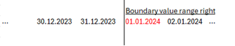
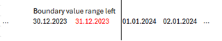
The partition function defines the range borders through boundary values and thus the number of partitions, in consideration with the data values, as well. You can define a partition function either as “range right” or “range left”. The main difference is how the boundary value gets treated. In a range right partition function, the boundary value is the first value of the next partition while in a range left partition function the boundary value is the last value of the previous partition. For example: 

We want to partition a table by year and the datatype of the column where we want to apply the partition function has the datatype “date”. Totally we have entries for the year 2023 and 2024 which means, we want 2x partitions. In a range right function, the boundary value must be the first day of the year 2024 whereas in a range left function the boundary value must be the last day of the year 2023.  

See example below: 

The partition scheme is used to map the different partitions, which are defined through the partition function, to multiple or one filegroup.

Main benefits of partitioning:

There are multiple scenarios where performance or manageability of a data model can be increased through partitioning. The main advantage of partitioning is that it reduces the contention on the whole table as a database object and restricts it to the partition level when performing operations on the corresponding data range. Partitioning also facilitates data transfer with the “switch partition” statement, this statement performs a switch-in or switch-out of o whole partition. Through that, a large amount of data can be transferred very quickly.

Demo Lab:

For demo purposes I created the following script, which will create three tables with 5 million rows of historical data from 11 years in the past until today:

USE [master] 
GO 
 
--Create Test Database 
CREATE DATABASE [TestPartition] 
GO 
 
--Change Recovery Model 
ALTER DATABASE [TestPartition] SET RECOVERY SIMPLE WITH NO_WAIT 
GO 
 
--Create Tables 
Use [TestPartition] 
GO 
 
CREATE TABLE [dbo].[Table01_HEAP]( 
[Entry_Datetime] [datetime] NOT NULL, 
[Entry_Text] [nvarchar](50) NULL 
) 
GO 
 
CREATE TABLE [dbo].[Table01_CLUSTEREDINDEX]( 
[Entry_Datetime] [datetime] NOT NULL, 
[Entry_Text] [nvarchar](50) NULL 
) 
GO 
 
CREATE TABLE [dbo].[Table01_PARTITIONED]( 
[Entry_Datetime] [datetime] NOT NULL, 
[Entry_Text] [nvarchar](50) NULL 
) 
GO 
 
--GENERATE DATA 
 
declare @date as datetime 
 
declare @YearSubtract int 
declare @DaySubtract int 
declare @HourSubtract int 
declare @MinuteSubtract int  
declare @SecondSubtract int  
declare @MilliSubtract int 
 
--Specifiy how many Years backwards data should be generated 
declare @YearsBackward int 
set @YearsBackward = 11 
 
--Specifiy how many rows of data should be generated 
declare @rows2generate int 
set @rows2generate = 5000000 
 
 
declare @counter int 
set @counter = 1 
 
--generate data entries 
while @counter <= @rows2generate  
begin 
 
--Year 
Set @YearSubtract = floor(rand() * (@YearsBackward - 0 + 1)) + 0 
--Day 
Set @DaySubtract = floor(rand() * (365 - 0 + 1)) + 0 
--Hour 
Set @HourSubtract = floor(rand() * (24 - 0 + 1)) + 0 
--Minute 
Set @MinuteSubtract = floor(rand() * (60 - 0 + 1)) + 0 
--Second 
Set @SecondSubtract = floor(rand() * (60 - 0 + 1)) + 0 
--Milisecond 
Set @MilliSubtract = floor(rand() * (1000 - 0 + 1)) + 0 
 
 
set @date = Dateadd(YEAR, -@YearSubtract , Getdate()) 
set @date = Dateadd(DAY, -@DaySubtract , @date) 
set @date = Dateadd(HOUR, -@HourSubtract , @date) 
set @date = Dateadd(MINUTE, -@MinuteSubtract , @date) 
set @date = Dateadd(SECOND, -@SecondSubtract , @date) 
set @date = Dateadd(MILLISECOND, @MilliSubtract , @date) 
 
insert into Table01_HEAP (Entry_Datetime, Entry_Text) 
Values (@date, 'This is a entry from ' + convert(nvarchar, @date, 29)) 
 
set @counter = @counter + 1 
 
end 
 
--COPY DATA TO OTHER TABLES 
 
INSERT INTO dbo.Table01_CLUSTEREDINDEX 
  (Entry_Datetime, Entry_Text) 
SELECT Entry_Datetime, Entry_Text 
  FROM Table01_HEAP 
 
INSERT INTO dbo.Table01_PARTITIONED 
  (Entry_Datetime, Entry_Text) 
SELECT Entry_Datetime, Entry_Text 
  FROM Table01_HEAP 
 
--Create Clustered Indexes for dbo.Table01_CLUSTEREDINDEX and dbo.Table01_PARTITIONED 
 
CREATE CLUSTERED INDEX [ClusteredIndex_Table01_CLUSTEREDINDEX] ON [dbo].[Table01_CLUSTEREDINDEX] 
( 
[Entry_Datetime] ASC 
 
) on [PRIMARY] 
GO 
 
CREATE CLUSTERED INDEX [ClusteredIndex_Table01_PARTITIONED] ON [dbo].[Table01_PARTITIONED] 
( 
[Entry_Datetime] ASC 
 
) on [PRIMARY] 
GO 

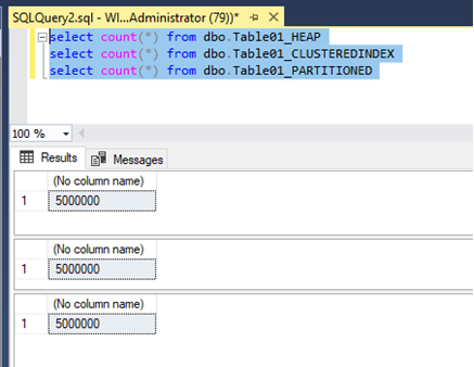
The tables have the same data in it. The difference between the tables is, that one is a heap, one has clustered index and one has a clustered Index which will be partitioned in the next step:

After the tables are created with the corresponding data and indexes, the partition function and scheme must be created. This was done by the following script:

-- Create Partition Function as range right for every Year -10 Years 
Create Partition Function [myPF01_datetime] (datetime) 
AS Range Right for Values ( 
DATEADD(yy, DATEDIFF(yy, 0, GETDATE()) + 0, 0), DATEADD(yy, DATEDIFF(yy, 0, GETDATE()) - 1, 0), DATEADD(yy, DATEDIFF(yy, 0, GETDATE()) - 2, 0), 
DATEADD(yy, DATEDIFF(yy, 0, GETDATE()) - 3, 0), DATEADD(yy, DATEDIFF(yy, 0, GETDATE()) - 4, 0), DATEADD(yy, DATEDIFF(yy, 0, GETDATE()) - 5, 0),  
DATEADD(yy, DATEDIFF(yy, 0, GETDATE()) - 6, 0), DATEADD(yy, DATEDIFF(yy, 0, GETDATE()) - 7, 0), DATEADD(yy, DATEDIFF(yy, 0, GETDATE()) - 8, 0),  
DATEADD(yy, DATEDIFF(yy, 0, GETDATE()) - 9, 0), DATEADD(yy, DATEDIFF(yy, 0, GETDATE()) - 10, 0) 
); 
GO 
 
-- Create Partition Scheme for Partition Function myPF01_datetime 
CREATE PARTITION SCHEME [myPS01_datetime] 
AS PARTITION myPF01_datetime ALL TO ([PRIMARY]) 
GO 

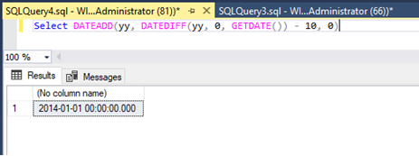
I have used the DATEADD() function in combination with the DATEDIFF() function to retrieve the first millisecond of the year as datetime data type and that for the last 10 years and used this as range right boundary values. For sure it is also possible to hard code the boundary values like ‘2014-01-01 00:00:00.000’ but I prefer to keep it as dynamically as possible. At the end it is the same result:

After creating the partition function, I have created the partition scheme. The partition scheme is mapped to the partition function. In my case I assign every partition to the primary filegroup. It is also possible to split the partitions across multiple filegroups.

As far as the partition function and scheme are created successfully it can be applied to the existing table: Table01_PARTITIONED. For achieving that, the clustered index of the table must be recreated on the partition scheme instead of the primary filegroup: 

-- Apply partitiononing on Table: Table01_PARTITIONED through recreating the Tables Clustered Index ClusteredIndex_Table01_PARTITIONED on Partition Scheme myPS01_datetime 
CREATE CLUSTERED INDEX [ClusteredIndex_Table01_PARTITIONED] ON [dbo].[Table01_PARTITIONED] 
( 
[Entry_Datetime] ASC 
 
) with (DROP_EXISTING = ON) on myPS01_datetime(Entry_Datetime);  
GO 

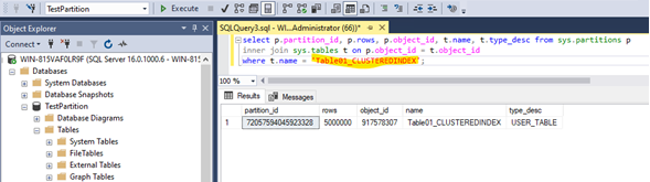
After doing that, the Table Table01_PARTITIONED has multiple partitions while the other tables have still only one partition: 

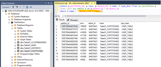
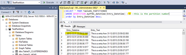
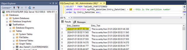
There are at all 12 partitions for every year between 2014 and 2024 as well as one for every entry which has an earlier datetime than 2014-01-01 00:00:00.000 and one for every entry that has a later datetime value than 2024-01-01 00:00:00.000 while partition nr. 1 has the earliest data and partition nr. 12 has the latest data in it. See below: 

DEMO Tests:

First, I want to compare the performance when moving outdated data, which is older than 2014-01-01 00:00:00.000, from the table itself to a history table. For that purpose, I created a history table with the same data structure as the table Table01_CLUSTEREDINDEX:

Use [TestPartition] 
GO 
 
--Create History Table 
CREATE TABLE [dbo].[Table01_HISTORY01]( 
[Entry_Datetime] [datetime] NOT NULL, 
[Entry_Text] [nvarchar](50) NULL 
) 
GO 
 
--Create Clustered Indexes for dbo.Table01_HISTORY01 
CREATE CLUSTERED INDEX [ClusteredIndex_Table01_HISTORY01] ON [dbo].[Table01_HISTORY01] 
( 
[Entry_Datetime] ASC 
 
) on [PRIMARY] 
GO 

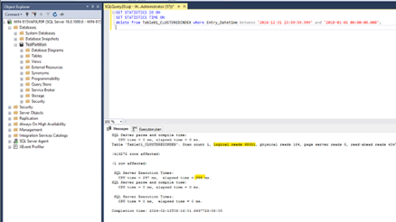
I am starting first with the table with the clustered index with a classic “insert into select” statement:

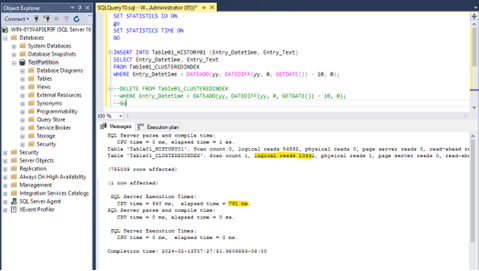
We can see that we have 10932 reads in total and a total query run time of 761 milliseconds.

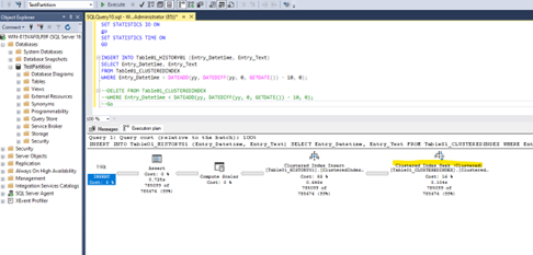
In the execution plan, we can see that a classical Index seek operation occurred. Which means, the database engine seeked for every row which has a datetime value previous to 2014-01-01 00:00:00.000 and wrote it into the history table.

For the delete operation we can see similar results:

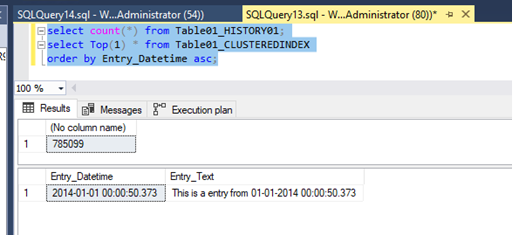
Totally 785099 rows where moved and we have in the table Table01_CLUSTEREDINDEX no older entries than 2014-01-01 00:00:00.000 anymore:

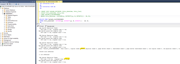
Next let us compare the data movement when using a “switch partition” statement. For switching a partition from a partitioned source table to a nonpartitioned destination table, we need to use the partition number of the source table. For that I run the following query:

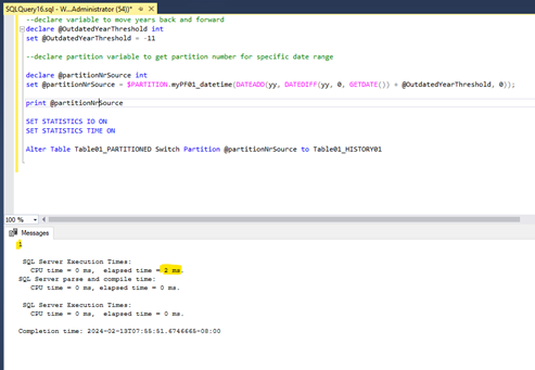
We can see that the partition number 1 was moved within 2 milliseconds. Compared to the previous query where it took 761 milliseconds for inserting the data and an additional 596 milliseconds for deleting the data, the switch partition operation is obviously much faster. But why is this the case? – that’s because switching partitions is a metadata operation. It does not seeking through an index (or even worse – scanning a table) and write every row one by one, instead it changes the metadata of the partition and remaps the partition to the target table. 

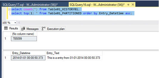
And as we can see, we have the same result:

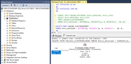
Another big advantage is when it comes to deleting a whole data range. For example: Let us delete the entries of the year 2017 – we do not need them anymore.

For the table with the clustered Index, we must use a statement like this:

We can see that we have here a query runtime of 355 milliseconds and 68351 page reads in total for the delete operation with the clustered index. 

For the partitioned table instead, we can use a truncate operation on the specific partition. That’s because the partition is treated as a own physical unit and can for that be truncated.

And as we should know: Truncating is much faster, because this operation is deallocating the pages and writes only one transaction log entry for the page deallocation while a delete operation is going row by row and writes every row deletion in the transaction log.

So, let us try: The year 2017 is 7 years back so let us verify, that the right data range will be deleted:

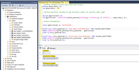
We can see with the short query above: 7 Years back, that would be the partition nr. 5 and the data range seems to be right.  So, let us truncate:

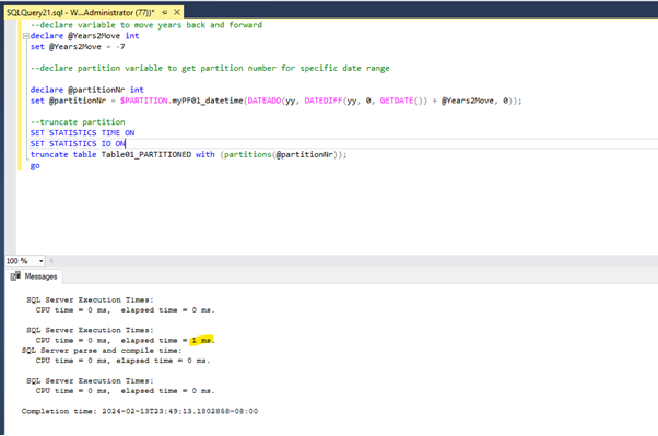
And we can see to truncate all the entries from the year 2017, the database engine took 1 millisecond compared to the 355 seconds for the delete operation again much faster.

Next: let’s see, how we can change the lock behavior of SQL-Server through partitioning. For that I ran the following update query for updating every entry text for dates which are younger than May 2018:

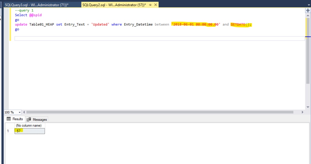
While the update operation above was running, I queried the DMV sys.dm_tran_locks in another session for checking the locks my update operation above is holding: 

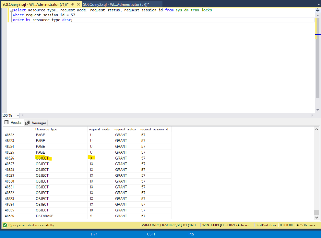
And we can see that we have a lot of page locks and also an exclusive lock on the object itself (in this case the Table01_HEAP).  That is because of SQL-Servers lock escalation behavior.

I ran the same update operation on the partitioned table but before I changed the lock escalation setting of the table from default value “table” to “auto”. This is necessary for enable locking on partition level: 

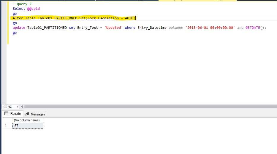
And when I’m querying the dmv again while the update operation above is running, I get the following result:

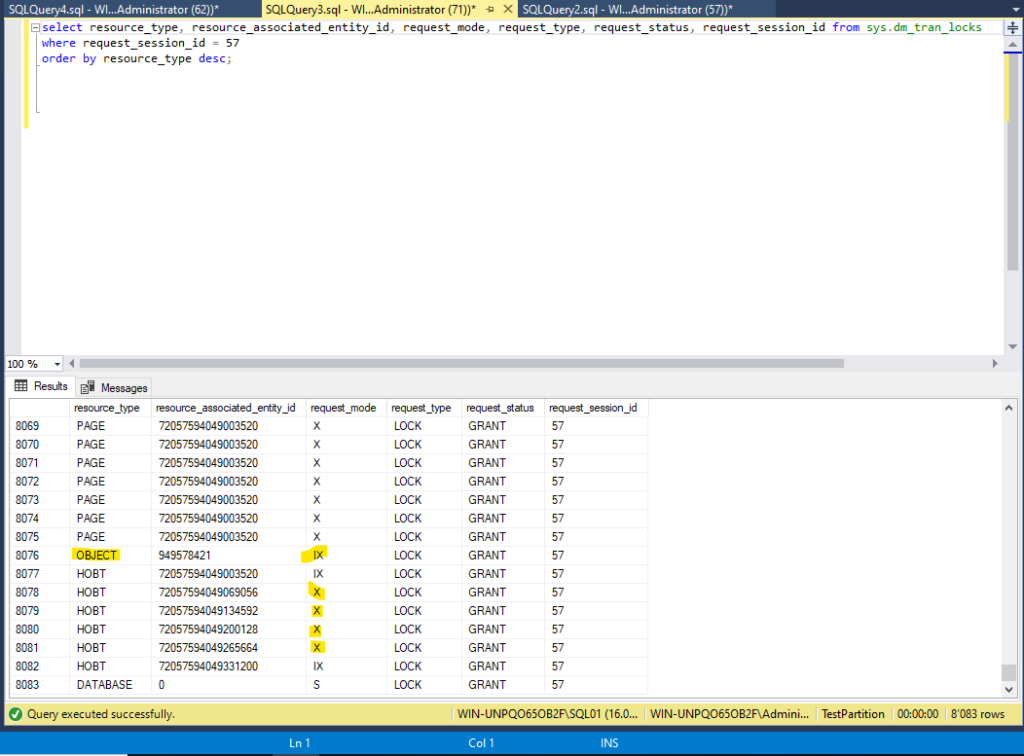
We can see that we have no exclusive look on abject level anymore, we have an intended exclusive look, which will not prevent other transactions from accessing the data (as far as it has no other look on a more granular level). Instead, we have multiple exclusive looks on multiple resources called HOBT. And when we take a look at the “resource_associated_entity_id” and using them for querying the sys.partitions table, we can see the following information’s: 

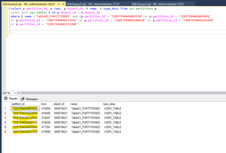
These resources locked through the update operation on the partitioned table are the partitions associated with the table. So, SQL-Server locked the partitions instead of locking the whole table. This has the advantage that locking happens in a more granular context which prevents lock contention on the table itself. 

Conclusion:

Partitioning can be a very powerful and useful functionality in SQL-Server when used in an appropriate situation. Especially when it comes to regular operations on whole data ranges, partitioning can be used for enhancing performance and manageability. With partitioning, it’s also possible to distribute the data of a table over multiple files groups. Additionally with splitting and merging partitions it’s possible to maintain partitions for growing or shrinking data.