This blog post follows the previous one about new direct seeding feature shipped with SQL Server 2016. As a reminder, I had some doubts about using direct seeding with large databases because log stream is not compressed by default but I forgot the performance improvements described into the Microsoft BOL. I also remembered to talk about it a couple of months ago in this blog post. So let’s try to combine all the things with the new direct seeding feature.
Microsoft did a good work of improving the AlwaysOn log transport layer and it could be very interesting to compare two methods: Adding a 100 GB database by using usual way that includes backup and restore operations from the primary to the secondary or using direct seeding feature. Which one is the quickest method?
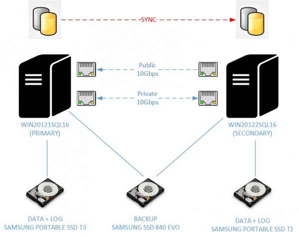
Let’s just have a quick look at my test environment. Two virtual machines with the following configuration:
- 4x Intel Core i7-3630QM 2.3 GHz
- 4GB of RAM
- 2 10Gbps network cards
- One disk that will host both the database data and log files on my primary replica (Samsung Portable SSD T3 500GB with S.M.A.R.T, NCQ and TRIM)
- One disk that will host both the database data and log files on my secondary replica (Samsung Portable SSD T1 500GB with S.M.A.R.T, NCQ and TRIM)
- One disk that will host backups (Samsung SSD 840 EVC, 250GB with S.M.A.R.T, NCQ and TRIM) used by both virtual machines
As an aside, each SSD disk is able to deliver at least 450MB/s and 35000 IOPS.
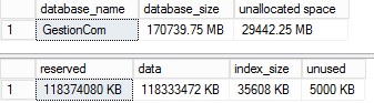
I also used a custom database named GestionCom that contains roughly 100GB of data for my test. 100GB would be sufficient to get relevant results.
Go ahead and let’s compare both synchronization methods
First test by using an usual way to add a database to an availability group
As said earlier, my first test will consist in using the usual way so far to add a database to an availability group. Let’s say that we may use 3 ways for data synchronization: FULL, join only and skip initial synchronization. We will use the first method for this test that includes all the steps: backup and restore the concerned database and then join it to the availability group. At this point we may easily image that the most part of the time will be consumed in the backup and restore step. I also want to precise that I did not use voluntary fine tuning options like BUFFERCOUNT, MAXTRANSFERSIZE or splitting backups to several media files in order to stay compliant with the availability group wizard.
| Step | Duration |
| Backup database to backup local disk (primary)WITH CHECKSUM, COMPRESSION | 06’55’’ |
| Restore database from network share (secondary)WITH CHECKSUM, NORECOVERY | 17’10’’ |
| Join database to availability group + start synchronization | 00’01’’ |
| Total | 24’06’’ |
What about resource consumption?
On the primary …
On the secondary …
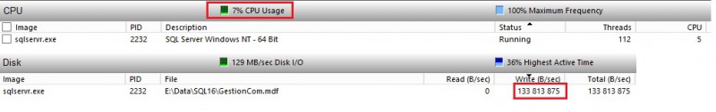
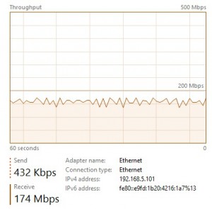
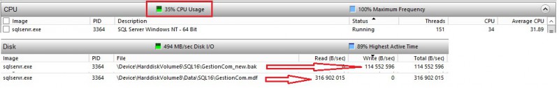
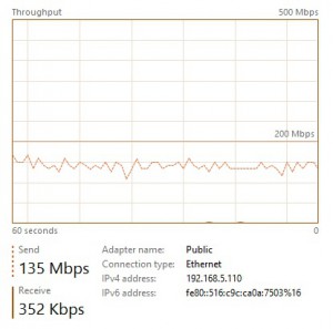
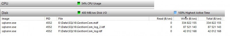
CPU utilization is equal to 35% on average during the test. Moreover, disk write throughput seems to stagnate to 130 MB/s on average and includes both backup and restore activities. The network throughput utilization seems also to stagnate between 135 Mbps and 174 Mbps according to my test.
So it is clear that my environment is under-used regarding resource consumption in this first test.
Second test by using new direct seeding method
This time I will use the new database deployment method: direct seeding. As said in my previous blog, using this feature will simplify a lot the adding database process but what about the synchronization speed and resource consumption in this case?
Well, to get a good picture of what happens during the seeding process, we will use different tools as the new sys.dm_hadr_automatic_seeding DMV and extended events as well. Extended events will help us to understand what happens under the cover in this case but to measure only the time duration of the operation we don’t need them. If you look at the event list as well as categories, you will probably notice a new dbseed category available that corresponds to the direct seeding. Events in this category are only available from the debug channel. That’s fine because we want to track when the seeding process starts, when it finishes and what’s happen between these two events (like failure, timeout, progress). By the way, the hadr_physical_progress may be very useful to get a picture of network activity for the concerned seeding session if your network card is shared between other sessions or availability group replication activities. In my case, I’m the only one and I will get this information directly from the task manager panel.
So let’s create the extended event session:
CREATE EVENT SESSION [hadr_direct_seeding]
ON SERVER
ADD EVENT sqlserver.hadr_automatic_seeding_start
(
    ACTION(sqlserver.database_name,sqlserver.sql_text)
	)
,
ADD EVENT sqlserver.hadr_automatic_seeding_state_transition
(
    ACTION(sqlserver.database_name,sqlserver.sql_text)
),
ADD EVENT sqlserver.hadr_automatic_seeding_success
(
    ACTION(sqlserver.database_name,sqlserver.sql_text)
),
ADD EVENT sqlserver.hadr_automatic_seeding_timeout
(
    ACTION(sqlserver.database_name,sqlserver.sql_text)
),
ADD EVENT sqlserver.hadr_physical_seeding_progress
(
    ACTION(sqlserver.database_name,sqlserver.sql_text)
)
ADD TARGET package0.event_file
(
	SET filename = N'hadr_direct_seeding',
	max_file_size = (2048),
	max_rollover_files = (10))
WITH
(
	MAX_MEMORY=4096 KB,
	EVENT_RETENTION_MODE = ALLOW_SINGLE_EVENT_LOSS,
	MAX_DISPATCH_LATENCY = 30 SECONDS,
	MAX_EVENT_SIZE = 0 KB,
	MEMORY_PARTITION_MODE = NONE,
	TRACK_CAUSALITY = OFF,
	STARTUP_STATE = OFF
)
GO
And after adding the GestionCom database to the TestGrp availability group, the direct seeding feature comes into play. Honestly, it was a very big surprise! Let’s take a look at the network utilization:
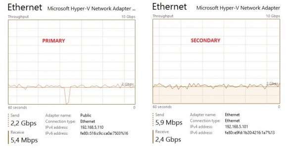
A network usage of 2.2 Gbps on average this time! The direct seeding feature provides a better use of the network bandwidth and we may understand clearly why efforts have been made by Microsoft to improve the synchronization process.
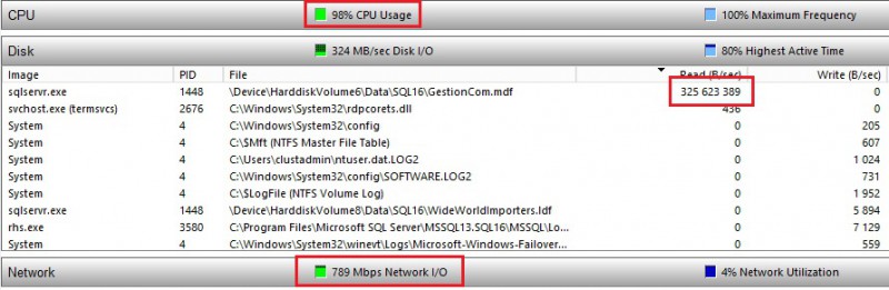
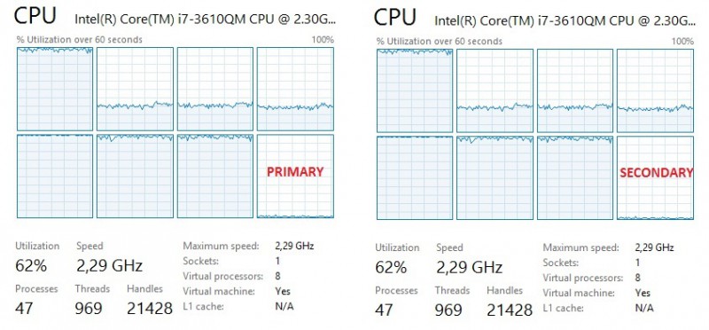
Let’s now move on the CPU and disk utilization respectively from the primary and then the secondary
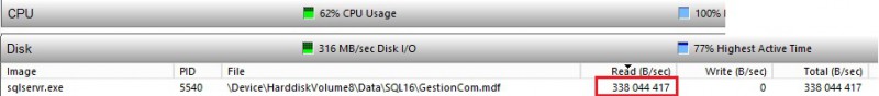
~ 350 up to 450 MB/s on each side (gain x2) but an increase of the CPU utilization up to 70% during my test (increase x2). So a better resource usage but at the cost of a higher CPU utilization …
Let’s finish by looking at the sys.dm_hadr_automatic_seeding DMV that provides the answer to the question: are we faster in this case?
select
    ag.name as aag_name,
    ar.replica_server_name,
    d.name as database_name,
    has.current_state,
    has.failure_state_desc as failure_state,
    has.error_code,
    has.performed_seeding,
	DATEADD(mi, DATEDIFF(mi, GETUTCDATE(), GETDATE()), has.start_time) as start_time,
	DATEADD(mi, DATEDIFF(mi, GETUTCDATE(), GETDATE()), has.completion_time) as completion_time,
    has.number_of_attempts
from sys.dm_hadr_automatic_seeding as has
join sys.availability_groups as ag
    on ag.group_id = has.ag_id
join sys.availability_replicas as ar
    on ar.replica_id = has.ag_remote_replica_id
join sys.databases as d
    on d.group_database_id = has.ag_db_id

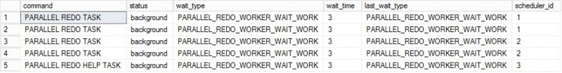
And the answer is yes as we may expect! Only 8 minutes (gain x3) to replicate and to synchronize the GestionCom database between the two high available replicas compared to the first method. But that’s not all … let’s focus on the redo thread activity from the secondary and you may notice a very interesting rate value (~ 12 MB/s). I don’t remember to have seen this value with current availability groups at customer places. This is the second improvement made by Microsoft concerned that has introduce parallel redo capability. As a reminder, before SQL Server 2016, there is only one redo thread per database. In this context, a single redo thread simply could not keep up with applying the changes as persisted in the log.
From the secondary, we may see some changes by looking at the sys.dm_exec_requests DMV:
select
	r.command,
	r.status,
	r.wait_type,
	r.wait_time,
	r.last_wait_type,
	r.scheduler_id
from sys.dm_exec_requests as r
where r.command like '%REDO%'
order by r.scheduler_id
Using direct seeding is definitely a solution to take into account to our future database deployment but I think we have to keep in mind two things according to this test: CPU and network consumption from seeding activity may impact the performance of other applications and vis-versa. In real world, there are good chances to be in this situation.
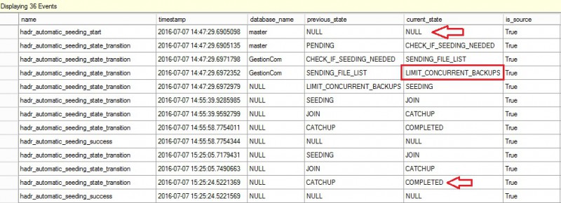
Finally let’s have a look at the extend event output. In respect of what we want to highlight in this blog post, we don’t get any other valuable information but one thing got my attention: LIMIT_CONCURRENT_BACKUPS value from the current value column (underlined in red). What does it mean exactly? Let’s talk about it in a next blog post because this is a little bit out of scope of the main subject.
Third test by using direct seeding and compression
Let’s talk about the last test I performed. I used direct seeding without compression in the previous test so SQL Server didn’t compress the data stream by default in this case. However we may force SQL Server to use compression by setting a special trace flag 9567. After all, we want to avoid direct seeding flooding the wire and impacting the existing workload from other applications.
I have to admit that enabling compression with direct seeding is not so obvious. For instance I didn’t see any difference from the DMVs that indicates we’re using compression. (is_compression_enabled column from the sys.dm_hadr_physical_seeding_stats DMV is always equal to 0 regardless we use or not compression). The only obvious difference comes from the network throughput usage that is lower with compression (gain x 2.5). However I noticed an important increase of CPU utilization near from 100% on the primary in my case.
What about seeding time? Well, I didn’t notice any gain on this field. Does compression allow to save network bandwidth? Maybe … hard to say with only this test and one specific environment.
I tried to add 3 VCPUs to each replica and leave one VCPU to the system so a total number of 7 VCPUS dedicated for SQL Server use.
At this point, I admit to be a little bit surprising and I wonder if compression uses correctly all the available processors regarding the uneven distribution of CPU resource usage. The above picture is a good representation of what I saw during other tests I performed with compression. In addition, I didn’t see any obvious performance gain in terms of duration except that wire is less used. I’m a little bit disappointed by compressiion but once again it is still much too early to draw a conclision and I’m looking forward direct seeding in action at my customers with real production infrastructure.
The bottom line is that direct seeding is a very promising feature and I love it because it is the direct visible part of the AlwaysOn performance improvements shipped with SQL Server 2016. However, and this is my personal opinion and not a recommandation, I think we don’t let it fool us and consider to use direct seeding carefully according to your workload and available resources. Fortunately, in most cases it will be suitable.
Stay tuned!
By David Barbarin
![Thumbnail [60x60]](https://www.dbi-services.com/blog/wp-content/uploads/2022/12/microsoft-square.png)
![Thumbnail [90x90]](https://www.dbi-services.com/blog/wp-content/uploads/2025/11/LTO_WEB.jpg)
![Thumbnail [90x90]](https://www.dbi-services.com/blog/wp-content/uploads/2023/01/APY_web-scaled.jpg)
![Thumbnail [90x90]](https://www.dbi-services.com/blog/wp-content/uploads/2022/08/FRJ_web-min-scaled.jpg)