Introduction
In this RAG series we tried so far to introduce new concepts of the RAG workflow each time. This new article is going to introduce also new key concepts at the heart of Retrieval. Adaptive RAG will allow us to talk about measuring the quality of the retrieved data and how we can leverage it to push our optimizations further.
A now famous study from MIT is stating how 95% of organizations fail to get ROI within the 6 months of their “AI projects”. Although we could argue about the relevancy of the study and what it actually measured, one of the key element to have a successful implementation is measurement.
An old BI principle is to know your KPI, what it really measures but also when it fails to measure. For example if you would use the speedometer on your dashboard’s car to measure the speed at which you are going, you’d be right as long as the wheels are touching the ground. So with that in mind, let’s see how we can create smart and reliable retrieval.
From Hybrid to Adaptive
Hybrid search significantly improves retrieval quality by combining dense semantic vectors with sparse lexical signals. However, real-world queries vary:
- Some are factual, asking for specific names, numbers, or entities.
- Others are conceptual, exploring ideas, reasons, or relationships.
A single static weighting between dense and sparse methods cannot perform optimally across all query types.
Adaptive RAG introduces a lightweight classifier that analyzes each query to determine its type and dynamically adjusts the hybrid weights before searching.
For example:
| Query Type | Example | Dense Weight | Sparse Weight |
|---|---|---|---|
| Factual | “Who founded PostgreSQL?” | 0.3 | 0.7 |
| Conceptual | “How does PostgreSQL handle concurrency?” | 0.7 | 0.3 |
| Exploratory | “Tell me about Postgres performance tuning” | 0.5 | 0.5 |
This dynamic weighting ensures that each search leverages the right signals:
- Sparse when exact matching matters.
- Dense when semantic similarity matters.
Under the hood, our AdaptiveSearchEngine wraps dense and sparse retrieval modules. Before executing, it classifies the query, assigns weights, and fuses the results via a weighted Reciprocal Rank Fusion (RRF), giving us the best of both worlds — adaptivity without complexity.
Confidence-Driven Retrieval
Once we make retrieval adaptive, the next challenge is trust. How confident are we in the results we just returned?
Confidence from Classification
Each query classification includes a confidence score (e.g., 0.92 “factual” vs 0.58 “conceptual”).
When classification confidence is low, Adaptive RAG defaults to a balanced retrieval (dense 0.5, sparse 0.5) — avoiding extreme weighting that might miss relevant content.
Confidence from Retrieval
We also compute confidence based on retrieval statistics:
- The similarity gap between the first and second ranked results (large gap = high confidence).
- Average similarity score of the top-k results.
- Ratio of sparse vs dense agreement (when both find the same document, confidence increases).
These metrics are aggregated into a normalized confidence score between 0 and 1:
def compute_confidence(top_scores, overlap_ratio):
    sim_conf = min(1.0, sum(top_scores[:3]) / 3)
    overlap_conf = 0.3 + 0.7 * overlap_ratio
    return round((sim_conf + overlap_conf) / 2, 2)
If confidence < 0.5, the system triggers a fallback strategy:
- Expands
top_kresults (e.g., from 10 → 30). - Broadens search to both dense and sparse equally.
- Logs the event for later evaluation.
The retrieval API now returns a structured response:
{
  "query": "When was PostgreSQL 1.0 released?",
  "query_type": "factual",
  "confidence": 0.87,
  "precision@10": 0.8,
  "recall@10": 0.75
}
This allows monitoring not just what was retrieved, but how sure the system is. Enabling alerting, adaptive reruns, or downstream LLM prompt adjustments (e.g., “Answer cautiously” when confidence < 0.6).
Evaluating Quality with nDCG
Precision and recall are fundamental metrics for retrieval systems, but they don’t consider the order of results. If a relevant document appears at rank 10 instead of rank 1, the user experience is still poor even if recall is high.
That’s why we now add nDCG@k (normalized Discounted Cumulative Gain) — a ranking-aware measure that rewards systems for ordering relevant results near the top.
The idea:
- DCG@k evaluates gain by position:
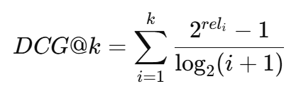
- nDCG@k normalizes this against the ideal order (IDCG):
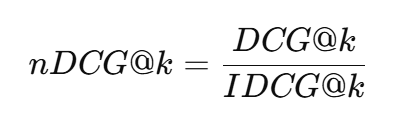
A perfect ranking yields nDCG = 1.0. Poorly ordered but complete results may still have high recall, but lower nDCG.
In practice, we calculate nDCG@10 for each query and average it over the dataset.
Our evaluation script (lab/04_evaluate/metrics.py) integrates this directly:
from evaluation import ndcg_at_k

score = ndcg_at_k(actual=relevant_docs, predicted=retrieved_docs, k=10)
print(f"nDCG@10: {score:.3f}")
Results on the Wikipedia dataset (25K articles)
| Method | Precision@10 | Recall@10 | nDCG@10 |
|---|---|---|---|
| Dense only | 0.61 | 0.54 | 0.63 |
| Hybrid fixed weights | 0.72 | 0.68 | 0.75 |
| Adaptive (dynamic) | 0.78 | 0.74 | 0.82 |
These results confirm that adaptive weighting not only improves raw accuracy but also produces better-ranked results, giving users relevant documents earlier in the list.
Implementation in our LAB
You can explore the implementation in the GitHub repository:
git clone https://github.com/boutaga/pgvector_RAG_search_lab
cd pgvector_RAG_search_lab
Key components:
lab/04_search/adaptive_search.py— query classification, adaptive weights, confidence scoring.lab/04_evaluate/metrics.py— precision, recall, and nDCG evaluation.- Streamlit UI (
streamlit run streamlit_demo.py) — visualize retrieved chunks, scores, and confidence in real time.
Example usage:
python lab/04_search/adaptive_search.py --query "Who invented SQL?"
Output:
Query type: factual (0.91 confidence)
Dense weight: 0.3 | Sparse weight: 0.7
Precision@10: 0.82 | Recall@10: 0.77 | nDCG@10: 0.84
This feedback loop closes the gap between research and production — making RAG not only smarter but measurable.
What is “Relevance”?
When we talk about precision, recall, or nDCG, all three depend on one hidden thing:
a ground truth of which documents are relevant for each query.
There are two main ways to establish that ground truth:
| Approach | Who decides relevance | Pros | Cons |
|---|---|---|---|
| Human labeling | Experts mark which documents correctly answer each query | Most accurate; useful for benchmarks | Expensive and slow |
| Automated or LLM-assisted labeling | An LLM (or rules) judges if a retrieved doc contains the correct answer | Scalable and repeatable | Risk of bias / noise |
In some business activity you are almost forced to use human labeling because the business technicalities are so deep that automating it is hard. Labeling can be slow and expensive for a business but I learned that it also is a way to introduce change management towards AI workflow by enabling key employees of the company to participate and build a solution with their expertise and without going through a harder project of asking to an external organization to create specific business logic into a software that was never made to handle it in the first place. As a DBA, I witnessed business logic move away from databases towards ORMs and application code and this time the business logic is going towards AI workflow. Starting this human labeling project my be the first step towards it and guarantees solid foundations.
Managers need to keep in mind that AI workflows are not just a technical solution, they are social-technical framework to allow organizational growth. You can’t just ship an AI chatbot into an app and expect 10x returns with minimal effort, this is a simplistic state of mind that already cost billions according the MIT study.
In a research setup (like your pgvector_RAG_search_lab), you can mix both approach:
- Start with a seed dataset of
(query, relevant_doc_ids)pairs (e.g. small set labeled manually). - Use the LLM to extend or validate relevance judgments automatically.
For example:
prompt = f"""
Query: {query}
Document: {doc_text[:2000]}
Is this document relevant to answering the query? (yes/no)
"""
llm_response = openai.ChatCompletion.create(...)
label = llm_response['choices'][0]['message']['content'].strip().lower() == 'yes'
Then you store that in a simple table or CSV:
| query_id | doc_id | relevant |
|---|---|---|
| 1 | 101 | true |
| 1 | 102 | false |
| 2 | 104 | true |
Precision & Recall in Practice
Once you have that table of true relevances, you can compute:
- Precision@k → “Of the top k documents I retrieved, how many were actually relevant?”
- Recall@k → “Of all truly relevant documents, how many did I retrieve in my top k?”
They’re correlated but not the same:
- High precision → few false positives.
- High recall → few false negatives.
For example:
| Query | Retrieved docs (top 5) | True relevant | Precision@5 | Recall@5 |
|---|---|---|---|---|
| “Who founded PostgreSQL?” | [d3, d7, d9, d1, d4] | [d1, d4] | 0.4 | 1.0 |
You got both relevant docs (good recall = 1.0), but only 2 of the 5 retrieved were correct (precision = 0.4).
Why nDCG is Needed
Precision and recall only measure which docs were retrieved, not where they appeared in the ranking.
nDCG@k adds ranking quality:
- Each relevant document gets a relevance grade (commonly 0, 1, 2 — irrelevant, relevant, highly relevant).
- The higher it appears in the ranked list, the higher the gain.
So if a highly relevant doc is ranked 1st, you get more credit than if it’s ranked 10th.
In your database, you can store relevance grades in a table like:
| query_id | doc_id | rel_grade |
|---|---|---|
| 1 | 101 | 2 |
| 1 | 102 | 1 |
| 1 | 103 | 0 |
Then your evaluator computes:
import math

def dcg_at_k(relevances, k):
    return sum((2**rel - 1) / math.log2(i+2) for i, rel in enumerate(relevances[:k]))

def ndcg_at_k(actual_relevances, k):
    ideal = sorted(actual_relevances, reverse=True)
    return dcg_at_k(actual_relevances, k) / dcg_at_k(ideal, k)
You do need to keep track of rank (the order in which docs were returned).
In PostgreSQL, you could log that like:
| query_id | doc_id | rank | score | rel_grade |
|---|---|---|---|---|
| 1 | 101 | 1 | 0.92 | 2 |
| 1 | 102 | 2 | 0.87 | 1 |
| 1 | 103 | 3 | 0.54 | 0 |
Then it’s easy to run SQL to evaluate:
SELECT query_id,
       SUM((POWER(2, rel_grade) - 1) / LOG(2, rank + 1)) AS dcg
FROM eval_results
WHERE rank <= 10
GROUP BY query_id;
In a real system (like your Streamlit or API demo), you can:
- Log each retrieval attempt (query, timestamp, ranking list, scores, confidence).
- Periodically recompute metrics (precision, recall, nDCG) using a fixed ground-truth set.
This lets you track if tuning (e.g., changing dense/sparse weights) is improving performance.
Structure of your evaluation log table could be:
| run_id | query_id | method | rank | doc_id | score | confidence | rel_grade |
|---|---|---|---|---|---|---|---|
| 2025-10-12_01 | 1 | adaptive_rrf | 1 | 101 | 0.92 | 0.87 | 2 |
| 2025-10-12_01 | 1 | adaptive_rrf | 2 | 102 | 0.85 | 0.87 | 1 |
From there, you can generate:
- nDCG@10 trend over runs (e.g., in Prometheus or Streamlit chart)
- Precision vs Confidence correlation
- Recall improvements per query type
⚠️ Note: While nDCG is a strong metric for ranking quality, it’s not free from bias. Because it normalizes per query, easier questions (with few relevant documents) can inflate the average score. In our lab, we mitigate this by logging both raw DCG and nDCG, and by comparing results across query categories (factual vs conceptual vs exploratory). This helps ensure improvements reflect true retrieval quality rather than statistical artifacts.
Human + LLM Hybrid Evaluation (Practical Middle Ground)
For your PostgreSQL lab setup:
- Label a small gold set manually (e.g., 20–50 queries × 3–5 relevant docs each).
- For larger coverage, use the LLM as an auto-grader.
You can even use self-consistency: ask the LLM to re-evaluate relevance twice and keep consistent labels only.
This gives you a semi-automated evaluation dataset, good enough to monitor:
- Precision@10
- Recall@10
- nDCG@10 over time
Lessons Learned
Through Adaptive RAG, we’ve transformed retrieval from a static process into a self-aware one.
- Precision increased by ~6–7%, especially for conceptual queries.
- Recall improved by ~8% for factual questions thanks to better keyword anchoring.
- nDCG@10 rose from 0.75 → 0.82, confirming that relevant results are appearing earlier.
- Confidence scoring provides operational visibility: we now know when the system is uncertain, enabling safe fallbacks and trust signals.
The combination of adaptive routing, confidence estimation, and nDCG evaluation makes this pipeline suitable for enterprise-grade RAG use cases — where explainability, reliability, and observability are as important as accuracy.
Conclusion and Next Steps
Adaptive RAG is the bridge between smart retrieval and reliable retrieval.
By classifying queries, tuning dense/sparse balance dynamically, and measuring ranking quality with nDCG, we now have a system that understands what kind of question it’s facing and how well it performed in answering it.
This version of the lab introduces the first metrics-driven feedback loop for RAG in PostgreSQL:
- Retrieve adaptively,
- Measure precisely,
- Adjust intelligently.
In the next part, we’ll push even further — introducing Agentic RAG, and how it plans and executes multi-step reasoning chains to improve retrieval and answer quality even more.
Try Adaptive RAG in the pgvector_RAG_search_lab repository, explore your own datasets, and start measuring nDCG@10 to see how adaptive retrieval changes the game.
![Thumbnail [60x60]](https://www.dbi-services.com/blog/wp-content/uploads/2025/03/OBA_web-scaled.jpg)
![Thumbnail [90x90]](https://www.dbi-services.com/blog/wp-content/uploads/2022/08/FRJ_web-min-scaled.jpg)