RAG Series – Naive RAG

Introduction

Since my last series on pgvector I had quite a fun time to work on RAG workflows on pgvector and learned some valuable lessons and decided to share some of it in a blog post series on the matter.
We will discover together where all RAG best practices are landing for the past 2 years and how can as a DBA or “AI workflow engineer” improve your designs to be production fit.
We start this series with Naïve RAG, this is quite known but important and foundational for the next posts of this series.

What is Retrieval-Augmented Generation (RAG)?

Retrieval-Augmented Generation (RAG) is a technique that combines the power of large language models (LLMs) with information retrieval. Instead of relying solely on an LLM’s internal knowledge (which may be outdated or limited, and prone to hallucinations), a RAG system retrieves relevant external documents and provides them as context for the LLM to generate a response. In practice, this means when a user asks a question, the system will retrieve a set of relevant text snippets (often from a knowledge base or database) and augment the LLM’s input with those snippets, so that the answer can be grounded in real data. This technique is key for integrating businesses or organizations data with LLMs capabilities because it allows you to implement business rules, guidelines, governance, data privacy constraints…etc.
Naïve RAG is the first logical step to understand how the retrieval part works and how it can impact the LLM output.

A RAG pipeline typically involves the following steps:

1. Document Embedding Storage – Your knowledge base documents are split into chunks and transformed into vector embeddings, which are stored in a vector index or database.
2. Query Embedding & Retrieval – The user’s query is converted into an embedding and the system performs a similarity search in the vector index to retrieve the top-$k$ most relevant chunks.
3. Generation using LLM – The retrieved chunks (as context) plus the query are given to an LLM which generates the final answer.

Try It Yourself

Clone the repository and explore this implementation:

git clone https://github.com/boutaga/pgvector_RAG_search_lab
cd pgvector_RAG_search_lab

The lab includes:

• Streamlit interface for testing different search methods
• n8n workflows for orchestrating the RAG pipeline
• Embedding generation scripts supporting multiple models
• Performance comparison tools to evaluate different approaches

Semantic Vector Search vs. Traditional SQL/Full-Text Search

Before diving deeper, it’s worth contrasting the vector-based semantic search used in RAG with traditional keyword-based search techniques (like SQL LIKE queries or full-text search indexes). This is especially important for DBAs who are familiar with SQL and may wonder why a vector approach is needed.

Traditional Search (SQL LIKE, full-text): Matches literal terms or boolean combinations. Precise for exact matches but fails when queries use different wording. A search for “car” won’t find documents about “automobiles” without explicit synonym handling.

Semantic Vector Search: Converts queries and documents into high-dimensional vectors encoding semantic meaning. Finds documents whose embeddings are closest to the query’s embedding in vector space, enabling retrieval based on context rather than exact matches.

The key advantage: semantic search improves recall when wording varies and excels with natural language queries. However, traditional search still has value for exact phrases or specific identifiers. Many production systems implement hybrid search combining both approaches (covered in a later post).

I am not going to go through all types of searches available in PostgreSQL but here is a diagram that is showing the historical and logical steps we went through the past decades.

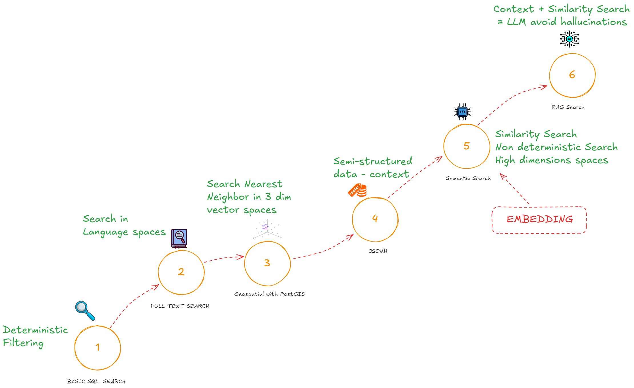
Key point: moving to vector search enables semantic retrieval that goes beyond what SQL LIKE or standard full-text indexes can achieve. It allows your RAG system to find the right information even when queries use different phrasing, making it far more robust for knowledge-based Q&A.

Building a Naïve RAG Pipeline (Step by Step)

Let’s break down how to implement a Naïve RAG pipeline properly, using the example from the pgvector_RAG_search_lab repository. We’ll go through the major components and discuss best practices at each step: document chunking, embedding generation, vector indexing, the retrieval query, and finally the generation step.

Here is a diagram of the entire data process :

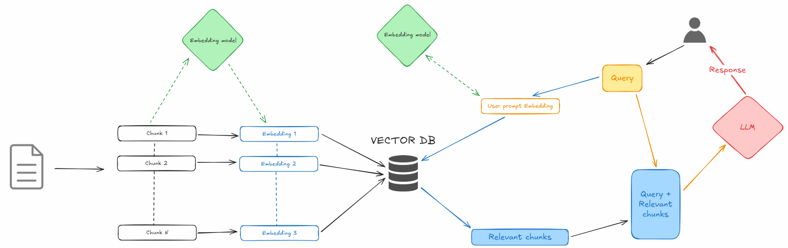
1. Document Ingestion – Chunking and Embeddings

Chunking documents: Large documents (e.g. long articles, manuals, etc.) need to be split into smaller pieces called chunks before embedding. Choosing the right chunking strategy is crucial. If chunks are too large, they may include irrelevant text along with relevant info; if too small, you might lose context needed to answer questions.

• Chunk size: test on your own data but a rule of thumb could be 100-150 tokens for factoid queries, 300+ for contextual queries but sentence or paragraph chunking are also an option.

Generating embeddings: Once the documents are chunked, each chunk is converted to a vector embedding by an embedding model. The choice of embedding model has a big impact on your RAG system’s effectiveness and is generally coupled with the LLM model you are going to choose. Since I am using ChatGPT-5, I went for OpenAI embedding models with 3072(large) and 1536(small) dimensions. The lab supports OpenAI’s text-embedding-3-large, small (dvdrental db) and open-source alternatives. Check MTEB benchmarks for model selection.

In the LAB repository you can generate the embeddings with the following Python script on the wikipedia database (Note: in the example bellow the SPLADE model is loaded but not used for dense vectors, the script is handling both dense and sparse embedding generation, we will cover this on the next blog post) :

(.venv) 12:56:43 postgres@PG1:/home/postgres/RAG_lab_demo/lab/embeddings/ [PG17] python generate_embeddings.py --source wikipedia --type dense
2025-09-27 12:57:28,407 - __main__ - INFO - Loading configuration...
2025-09-27 12:57:28,408 - __main__ - INFO - Initializing services...
2025-09-27 12:57:28,412 - lab.core.database - INFO - Database pool initialized with 1-20 connections
2025-09-27 12:57:29,093 - lab.core.embeddings - INFO - Initialized OpenAI embedder with model: text-embedding-3-large
2025-09-27 12:57:33,738 - lab.core.embeddings - INFO - Loading SPLADE model: naver/splade-cocondenser-ensembledistil on device: cpu
Some weights of BertModel were not initialized from the model checkpoint at naver/splade-cocondenser-ensembledistil and are newly initialized: ['pooler.dense.bias', 'pooler.dense.weight']
You should probably TRAIN this model on a down-stream task to be able to use it for predictions and inference.
2025-09-27 12:57:34,976 - lab.core.embeddings - INFO - SPLADE embedder initialized on cpu

============================================================
EMBEDDING GENERATION JOB SUMMARY
============================================================
Source: wikipedia
Embedding Type: dense
Update Existing: False
============================================================

CURRENT STATUS:
Wikipedia Articles: 25000 total, 25000 with title embeddings
                   25000 with content embeddings

Proceed with embedding generation? (y/N): y

============================================================
EXECUTING JOB 1/1
Table: articles
Type: dense
Columns: ['title', 'content'] -> ['title_vector_3072', 'content_vector_3072']
============================================================
2025-09-27 12:57:41,367 - lab.embeddings.embedding_manager - INFO - Starting embedding generation job: wikipedia - dense
2025-09-27 12:57:41,389 - lab.embeddings.embedding_manager - WARNING - No items found for embedding generation

Job 1 completed:
  Successful: 0
  Failed: 0

============================================================
FINAL SUMMARY
============================================================
Total items processed: 0
Successful: 0
Failed: 0

FINAL EMBEDDING STATUS:

============================================================
EMBEDDING GENERATION JOB SUMMARY
============================================================
Source: wikipedia
Embedding Type: dense
Update Existing: False
============================================================

CURRENT STATUS:
Wikipedia Articles: 25000 total, 25000 with title embeddings
                   25000 with content embeddings
2025-09-27 12:57:41,422 - __main__ - INFO - Embedding generation completed successfully
2025-09-27 12:57:41,422 - lab.core.database - INFO - Database connection pool closed
(.venv) 12:57:42 postgres@PG1:/home/postgres/RAG_lab_demo/lab/embeddings/ [PG17]

After these steps, you will have a vectorized database: each document chunk is represented by a vector, stored in a table (if using a DB like Postgres/pgvector) or in a vector store. Now it’s ready to be queried.

2. Vector Indexing and Search in Postgres (pgvector + DiskANN)

For production-scale RAG, how you index and search your vectors is critical for performance. In a naive setup, you might simply do a brute-force nearest neighbor search over all embeddings – which is fine for a small dataset or testing, but too slow for large collections. Instead, you should use an Approximate Nearest Neighbor (ANN) index to speed up retrieval. The pgvector extension for PostgreSQL allows you to create such indexes in the database itself.

Using pgvector in Postgres: pgvector stores vectors and supports IVFFlat and HNSW for ANN. For larger-than-RAM or cost-sensitive workloads, add the pgvectorscale extension, which introduces a StreamingDiskANN index inspired by Microsoft’s DiskANN, plus compression and filtered search.

! Not all specialized Vector databases or Vector stores have this feature, if your data needs to scale this is a critical aspect !

For our Naïve RAG example :

CREATE INDEX idx_articles_content_vec
ON articles
USING diskann (content_vector vector_cosine_ops);

Why use Postgres for RAG? For many organizations, using Postgres with pgvector is convenient because it keeps the vectors alongside other relational data and leverages existing operational familiarity (backup, security, etc.). It avoids introducing a separate vector database. Storing vectors in your existing operational DB can eliminate the complexity of syncing data with a separate vector store, while still enabling semantic search (not just keyword search) on that data. With extensions like pgvector (and vectorscale), Postgres can achieve performance close to specialized vector DBs, if not better. Of course, specialized solutions (Pinecone, Weaviate, etc.) are also options – but the pgvector approach is very appealing for DBAs who want everything in one familiar ecosystem.

3. Query Processing and Retrieval

With the data indexed, the runtime query flow of Naïve RAG is straightforward:

• Query embedding: When a user question comes in (for example: “What is WAL in PostgreSQL and why is it important?”), we first transform that query into an embedding vector using the same model we used for documents. This could be a real-time call to an API (if using an external service like OpenAI for embeddings) or a local model inference. Caching can be applied for repeated queries, though user queries are often unique. Ensure the text of the query is cleaned or processed in the same way document text was (e.g., if you did lowercasing, removal of certain stopwords, etc., apply consistently if needed – though modern embedding models typically handle raw text well without special preprocessing).
• Vector similarity search: We then perform the ANN search in the vector index with the query embedding. As shown earlier, this is an ORDER BY vector <=> query_vector LIMIT k type query in SQL (or the equivalent call in your vector DB’s client). The result is the top k most similar chunks to the query. Choosing k (the number of chunks) to retrieve is another design parameter: common values are in the range 3–10. You want enough pieces of context to cover the answer, but not so many that you overwhelm the LLM or introduce irrelevant noise. A typical default is k=5. In the example lab workflow, they use a top_k of 5 by default. If you retrieve too few, you might miss part of the answer; too many, and the prompt to the LLM becomes long and could confuse it with extraneous info.

The outcome of the retrieval step is a set of top-k text chunks (contexts) that hopefully contain the information needed to answer the user’s question.

4. LLM Answer Generation

Finally, the retrieved chunks are fed into the prompt of a large language model to generate the answer. This step is often implemented with a prompt template such as:

“Use the following context to answer the question. If the context does not have the answer, say you don’t know.
Context:
[Chunk 1 text]
[Chunk 2 text]
…
Question: [User’s query]
Answer:”

The LLM (which could be GPT-5, or an open-source model depending on your choice) will then produce an answer, hopefully drawing facts from the provided context rather than hallucinating. Naïve RAG doesn’t include complex prompt strategies or multiple prompt stages; it’s usually a single prompt that includes all top chunks at once (this is often called the “stuffing” approach – stuffing the context into the prompt). This is simple and works well when the amount of context is within the model’s input limit.

Best practices for the generation step:

• Order and formatting of contexts: Usually, chunks can be simply concatenated. It can help to separate them with headings or bullet points, or any delimiter that clearly resets context. Some frameworks sort retrieved chunks by similarity score (highest first) under the assumption that the first few are most relevant – this makes sense so that if the prompt gets truncated or the model gives more weight to earlier context (which can happen), the best info is first.
• Avoid exceeding token limits: If each chunk is, say, ~100 tokens and you include 5 chunks, that’s ~500 tokens of context plus the prompt overhead and question. This should fit in most LLMs with 4k+ token contexts. But if your chunks or k are larger, be mindful not to exceed the model’s max token limit for input. If needed, reduce k or chunk size, or consider splitting the question into sub-queries (advanced strategy) to handle very broad asks.
• Prompt instructions: In naive usage, you rely on the model to use the context well. It’s important to instruct the model clearly to only use the provided context for answering, and to indicate if the context doesn’t have the answer. This mitigates hallucination. For example, telling it explicitly “If you don’t find the answer in the context, respond that you are unsure or that it’s not in the provided data.” This way, if retrieval ever fails (e.g., our top-k didn’t actually contain the needed info), the model won’t fabricate an answer. It will either abstain or say “I don’t know.” Depending on your application, you might handle that case by maybe increasing k or using a fallback search method.
• Citing sources: A nice practice, especially for production QA systems, is to have the LLM output the source of the information (like document titles or IDs). Since your retrieval returns chunk metadata, you can either have the model include them in the answer or attach them after the fact. This builds trust with users and helps for debugging. For instance, the lab workflow tracks the titles of retrieved articles and could enable showing which Wikipedia article an answer came from. In a naive setup, you might just append a list of sources (“Source: [Title of Article]”) to the answer.

With that, the Naïve RAG pipeline is complete: the user’s query is answered by the LLM using real data fetched from your database. Despite its simplicity, this approach can already dramatically improve the factual accuracy of answers and allow your system to handle queries about information that the base LLM was never trained on (for example, very recent or niche knowledge).

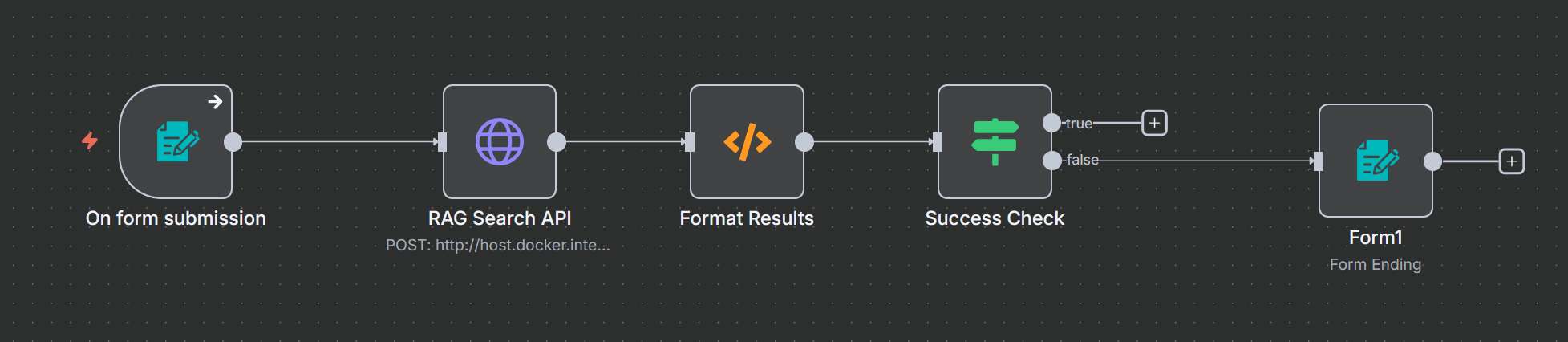
In our LAB setup on n8n the workflow without the chunking and embedding generation looks like that :
Note that we use

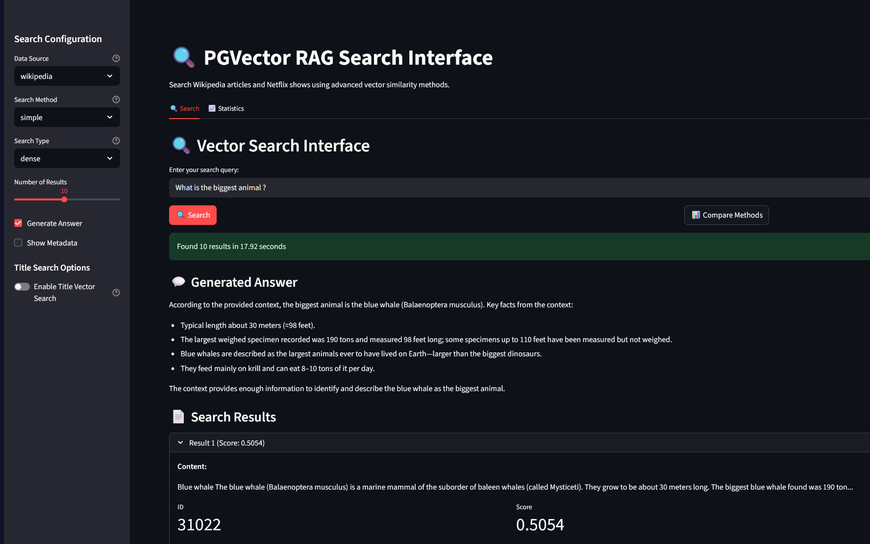
In the Streamlit interface also provided in the repo, we have the following :

Monitoring and Improving RAG in Production

Implementing the pipeline is only part of the story. In a production setting, we need to monitor the system’s performance and gather feedback to continuously improve it.
The comparison workflow allows side-by-side testing of:

• Different embedding models
• Chunk sizes and strategies
• Retrieval parameters (top-k values)
• LLM prompting approaches

In summary, treat your RAG system as an evolving product: monitor retrieval relevance, answer accuracy (groundedness), and system performance. Use a combination of automated metrics and human review to ensure quality. Tools like LangSmith can provide infrastructure for logging queries and scoring outputs on metrics like faithfulness or relevance, flagging issues like “bad retrievals” or hallucinated responses. By keeping an eye on these aspects, you can iterate and improve your Naïve RAG system continuously, making it more robust and trustworthy. Although Langsmith is very usefull, be carefull with the necessary pitfall that come along with any abstraction. A good rule of thumb would be to keep your core logic into custom code while taking leverage of Langsmith tools for peripherals.

Conclusion and Next Steps

Naïve RAG provides the basic blueprint of how to augment LLMs with external knowledge using semantic search. We discussed how to implement it using PostgreSQL with pgvector, covering best practices in chunking your data, selecting suitable embeddings, indexing with advanced methods like DiskANN for speed, and ensuring that you monitor the system’s effectiveness in production. This straightforward dense retrieval approach is often the first step toward building a production-grade QA system. It’s relatively easy to set up and already yields substantial gains in answer accuracy and currency of information.

However, as powerful as Naïve RAG is, it has its limitations. Pure dense vector similarity can sometimes miss exact matches (like precise figures or rare terms) that a keyword search would catch, and it might bring in semantically relevant but not factually useful context in some cases. In the upcoming posts of this series, we’ll explore more advanced RAG techniques that address these issues:

• Hybrid RAG: combining dense vectors with sparse (lexical) search to get the best of both worlds – we’ll see how a hybrid approach can improve recall and precision by weighting semantic and keyword signals GitHub.
• Adaptive RAG: introducing intelligent query classification and dynamic retrieval strategies – for example, automatically detecting when to favor lexical vs. semantic, or how to route certain queries to specialized retrievers.
• and other more trendy RAG types like Self RAG or Agentic RAG….

As you experiment with the provided lab or your own data, remember the core best practices: ensure your retrieval is solid (that often solves most problems), and always ground the LLM’s output in real, retrieved data. The repository will introduce other RAG and lab examples over time, the hybrid and adaptive workflows are already built in though.
With all the fuss around AI and LLM it might seem chaotic from an outsider with a lack of stability and maturity. There a good chance that the RAG fundamental component will still be there in the coming years if not decade, it lasted 2 years already and proved useful, we just might see those components be summed and integrated to other systems especially with components provided normative monitoring and evaluation which the big open subject. We can’t say that RAG patterns we have are mature but we know for sure they are fundamental to what is coming next.

Stay tuned for the next part, where we dive into Hybrid RAG and demonstrate how combining search strategies can boost performance beyond what naive semantic search can do alone.